Algorithmic complexity
Contents
Algorithmic complexity#
In order to make our programs efficient (or, at least, not horribly inefficient), we can consider how the execution time varies depending on the input size \(n\). Let us define a measure of this efficiency as a function \( T(n)\). Of course, the time it takes to execute a code will vary largely depending on the processor, compiler or disk speed. \( T(n)\) goes around this variance by measuring asymptotic complexity. In this case, only (broadly defined) steps will determine the time it takes to execute an algorithm.
Now, say we want to add two \(n\)-bit binary digits. One way to do this is to go bit by bit and add the two. We can see that \(n\) operations are involved.
where \(c\) is the time it takes to add two bits on a machine. On different machines, the value of \(c\) may vary, but the linearity of this function is the common factor. Our aim is to abstract away from the details of implementation and think about the fundamental usage of computing resources.
Big O notation#
The mathematical definiton of this concept can be found here. In simple terms, we say that:
if there exists \(c>0\) and \(n_0>0\) such that
\(g(n)\) can be thought of as an upper bound of \(f(n)\) as \(n \to \infty\). In some publications big Theta notation is used. \(\Theta(n)\) can be considered the least upper bound, in algorithm analysis we ofter use both notations interchangeably.
Here are a couple of examples:
but also:
We will now consider different time complexities of algorithms.
Constant time \(O(1)\)#
An algorithm is said to run in constant time if its complexity is \(O(1)\). This is usually considered the fastest case (which is true but only in the asymptotic sense). No matter what the input size is, the program will take the same amount of time to terminate. Let us consider some examples:
Hello World!:
def f(n):
    print("Hello World!")
No matter what n is, the function does the same thing, which takes the same time. Therefore its complexity is constant.
Checking if an integer is odd or not:
import time

def f(n):
    return n & 1 == 1
print(f(7))
print(f(2349017324987123948729382))
True
False
In this case, we only need to check if the zeroth bit of the binary representation is set to 1. The number of operations does not depend on the value or the size of the input number.
Searching a dictionary:
d = {}
d['A'] = 1
d['B'] = 2
d['C'] = 3

print(d['B'])
2
Dictionaries are data structures which can be queried in constant time. If we have a key, we can retrieve an element instantaneously.
Linear time \(O(n)\)#
This complexity appears in real-life problems much more frequently than constant time. The program is said to run in linear time if the time it takes is proportional to the input size:
Finding a maximum in an unsorted list:
def f(l):
    _max = l[0]
    for i in l:
        if i > _max:
            _max  = i
    return _max

print(f([1,4,7,4,3,9,0,4,-3]))
9
As we do not know anything about the order of elements in this list, we need to check every element in order to see if it is not the greatest. The longer the list, the more such checks are needed. In general, when we need to go trough some data structure a constant number of times, we are dealing with linear time.
Quadratic time \(O(n^2)\)#
The quadratic time complexity is also a very popular case. It often might not be the most efficient solution and can point to better complexities such as \(O(n*\log(n))\). However, there are problems in which such traversal is necessary.
Selection sort:
def swap(i,j,l):
    temp = l[i]
    l[i] = l[j]
    l[j] = temp

def selectionSort(l):

    i = 0

    while i < len(l)-1:
        swap(i,i+l[i:].index(min(l[i:])),l)
        i+=1

    return l

print(selectionSort([3,4,5,6,7,8,9,3,2]))
[2, 3, 3, 4, 5, 6, 7, 8, 9]
The algorithm works as follows:
Find the minimum of the list and swap it with the first element.
Now consider all elements behind the first index
Find the minimum of this sublist and swap it with the first element (of the sublist)S
A diagram says more than a 1000 words:
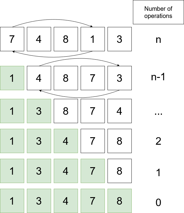
If we calculate the sum of operations (arithmetic series) we get \(\frac{n*(n+1)}{2} = O(n^2)\). Selection Sort is considered a rather inefficient sorting algorithm.
Adding Matrices:
# Adds two square matrices of the same size
def addMatrix(A,B):
    res = []
    for i in range(len(A)):
        temp = []
        for j in range(len(A[i])):

            temp.append(A[i][j] + B[i][j])

        res.append(temp)

    return res


print(addMatrix([[1,2,3],[1,2,3],[1,2,3]],[[3,2,1],[3,2,1],[3,2,1]]))
[[4, 4, 4], [4, 4, 4], [4, 4, 4]]
When we want to add two \(n \times n\) matrices, we have to perform the addition element-wise, therefore we perform \(n^2\) additions.
Different complexities#
Apart from the three complexities above, there are many more which show up quite often. The most notable ones are (we will discuss some of them later):
Logarithmic \(O(\log(n))\) - present in e.g. Binary Search.
Loglinear \(O(n*\log(n))\) - e.g. Merge Sort.
Multi-variable \(O(n*k)\) - e.g. searching for a substring of length \(k\) in a string of length \(n\).
Exponential \(O(a^n)\), \(a > 1\) - this is bad.
Factorial \(O(n!)\) - even worse (producing all permutations of a string).
Best, worst and average case runtimes#
While analyzing algorithms, it is worth considering how the program behaves based on different inputs.
Best-case runtime complexity is a function defined by the minimum number of steps taken on any input.
Worst-case runtime complexity considers the maximum number of steps taken by the algorithm.
Average case runtime complexity is probably the most accurate measure of the performance of an algorithm and takes into account the behaviour of the program when fed with an average input.
In production, both worst and average runtime complexities are considered (imagine an algorithm with an average \(O(n^2)\) and worst-case \(O(n!)\) - that could be easily exploited!)
Let us now perform an analysis on a simple search algorithm which finds the number \(x\) in a list \(l\)
def simpleSearch(x,l):
    for i in range(len(l)):
        if x == l[i]:
            return i
    return -1

print(simpleSearch(1,[3,4,5,6,7,1,23,4]))
5
Our assumption is that \(x\) is in the list and that the probability that it is at a particular index is uniform.
Best-case: \(O(1)\) - in is the zeroth cell
Worst-case: \(O(n)\) - have to go through the whole list
Average case: \(O(\frac{n}{2}) = O(n)\) - the element will be somewhere in the middle
In this case, we can predict that the program will run in linear time.
Exercises#
Which Big O category do these functions fall into (least upper bound):
\( 4n^3 + 2n\)
\(\sum_{i=0}^{n} i^2\)
\(\log(\log(n))\)
34562
Answers
\(O(n^3)\)
\(O(n^3)\)
\(O(\log(\log(n))\)
\(O(1)\)
Multiplying Matrices We want to multiply two square matrices of side length \(n\) of the same size using the following code:
def mulMatrix(A,B):

    C = [([0]*len(A)) for i in range(len(A))]

    for i in range(len(A)):
        for j in range(len(A)):
            for k in range(len(A)):
                C[i][j] += (A[i][k]*B[k][j])

    return C


print(mulMatrix([[1,1,1],[2,2,2],[3,3,3]],
                [[1,2,3],[1,2,3],[1,2,3]]))
[[3, 6, 9], [6, 12, 18], [9, 18, 27]]
What is the algorythmic complexity of this algorithm?
Answer
The function mulMatrix in its innermost loop does two operations: one multiplication and one addition. It does this \(n^3\) times because there are three nested for loops, each one iterating n times.
Therefore \(O(n^3)\).
Insertion Sort algorithm works according to the steps:
Take the minimum element from the list and swap it with the first element.
Now elements before index 1 are sorted
Take the minimum element from the unsorted portion of the list and put it at an appropriate position in the sorted portion.
Repeat until the whole list is sorted.
The following GIF should be helpful:

Source: Wikimedia Commons
What is the algorythmic complexity of this algorithm?
Answer
\(O(n^2)\)
References#
Victor S.Adamchik, CMU, 2009 Algorythmic Complexity
Adrian Mejia, Medium, 2018 8 time complexity examples that every programmer should know