Euler Pole
Contents
Euler Pole#
Pure Geophysics Continental Tectonics
Kinematics of Plate Tectonics#
Plates drift through time. An important part of what Bullard et al. did was to show that the conjugate margins of Africa and South America could be fit together using Euler’s fixed point theorem.
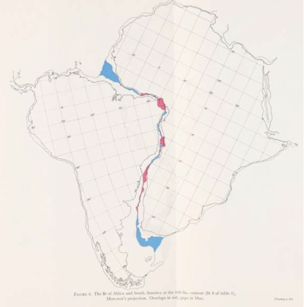
Bullard et al. determined the Euler pole and finite rotation that best manages to bring the two margins (the ∼\(1\,km\) bathymetric contour on both margins) together. Amazingly most of the margins of these two continents can be fit together using a single rotation about a single Euler pole. Their results played an important role in bridging the gap between rather qualitative ideas about continental drift (which were highly controversial at the time) and plate tectonic theory as we now know it. Perhaps more amazingly they did most of this work as marine geophysics was just getting going and very little was known about the shapes of the ocean basins.
Euler’s fixed point theorem#
First we need to define the position of the Euler pole about which we are going to perform the rotation (i.e. its longitude, \({\theta}_{e}\), and latitude, \({\lambda}_{e}\)). Secondly, we need to define the finite rotation \(e\). You could visualise the resultant vectors of motion on Earth’s surface as small circles centred on the Euler pole (e.g. Figure 2).
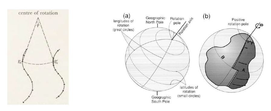
Figure 2: Left panel shows rotation of points about a centre of rotation. Dashed line connecting points \(P_{n}\) and \(P'_{n}\) = small circle (i.e. the path the point takes as it rotates). Right panels show Euler poles (i.e. poles of rotation) with associated small circles (along which translation of points occurs) atop three dimensional representations of the Earth. Note that the pole of rotation is not necessarily a geographic or magnetic pole. Rightmost panel shows an example of two plates A and B having moved apart with a finite rotation \({\omega}\). Note that the distance between the plates increases with distance away from the pole and that here we are considering finite rotations and not angular velocities.
Translation of points along great circles#
To calculate the movement of any point on Earth’s surface from its starting point, \(P\), to its rotated position \(P′\), we first need to know how far away the starting point is from the Euler pole. We can use spherical trigonometry and the spherical law of cosines to calculate this distance, \(d\), such that:
where \({\lambda}_{p}\) and \({\lambda}_{e}\) are the latitudes of the starting point and the Euler pole, respectively and \({\Delta}{\theta}\) is the absolute difference between the two longitudes (hint: work in radians, \(\pi\,rad = 180^\circ\)). We can now use these values to calculate the angular distance, \({\omega}'\), between the starting and rotated point (i.e. how far the point has moved as a function of the rotation about the Euler pole). Using the law of cosines,
Note that we have assumed that the distance from the pole to the rotated and unrotated points is the same. Now after all that we are ready to calculate the position of the rotated point.
Positions of rotated points#
For convenience we are first going to convert spherical coordinates to cartesian coordinates,