Fourier series in Python

Mathematics Methods 2 Mathematics for Scientists and Engineers 1 Waves

In this notebook, Python will be used to calculate and generate these Fourier series and transforms.

Waves of any shape can be modelled and described using Fourier series.

The general Fourier series is of the form:

\[y(t) = \frac{a_0}{2} + \sum_{n=1}^{\infty} a_n \sin(n\omega t) +\sum_{m=1}^{\infty} b_m \sin(m\omega t) \]

Here,

\[a_0 = \frac{2}{\tau} \int_{0}^{\tau} y(t) \,dt\]

\[a_n = \frac{2}{\tau} \int_{0}^{\tau} y(t)\sin(n\omega t) \,dt\]

\[b_m = \frac{2}{\tau} \int_{0}^{\tau} y(t)\cos(m\omega t) \,dt\]

Where \(\tau\) is the period.

import sympy as sym
from sympy import pi
import matplotlib.pyplot as plt
from scipy.signal import square
import numpy as np
import scipy.integrate as integrate
from scipy import fftpack

Finding Fourier components

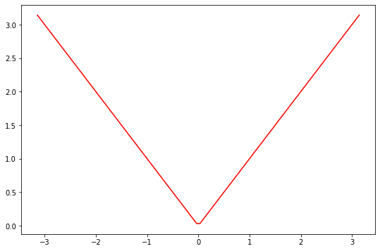
def triangle(x):
    if x>=0:
        return x
    else:
        return -x

def fourier(function, lower_limit, upper_limit, number_terms):
    l = (upper_limit-lower_limit)/2
    a0=1/l*integrate.quad(lambda x: function(x), lower_limit, upper_limit)[0]
    A = np.zeros((number_terms))
    B = np.zeros((number_terms))
     
    for i in range(1,number_terms+1):
        A[i-1]=1/l*integrate.quad(lambda x: function(x)*np.cos(i*np.pi*x/l), lower_limit, upper_limit)[0]
        B[i-1]=1/l* integrate.quad(lambda x: function(x)*np.sin(i*np.pi*x/l), lower_limit, upper_limit)[0]
 
    return [a0/2.0, A, B]

# plot triangle function
plt.figure(figsize=(9,6)) 
x = np.linspace(-np.pi, np.pi, 100)
triangle_values = [triangle(item) for item in x]
plt.plot(x, triangle_values, 'r')

[<matplotlib.lines.Line2D at 0x7f9ee5ddbbe0>]

traingle_coeffs = fourier(triangle, -np.pi, np.pi, 3)
print('Fourier coefficients for the Triangular wave for three harmonic numbers\n')
print('a0 ='+str(traingle_coeffs[0]))
print('an ='+str(traingle_coeffs[1]))
print('bn ='+str(traingle_coeffs[2]))

Fourier coefficients for the Triangular wave for three harmonic numbers

a0 =1.5707963267948966
an =[-1.27323954e+00  4.99600361e-16 -1.41471061e-01]
bn =[0. 0. 0.]

Finding Fourier series using sympy module

L=10
x=np.arange(-L,L,0.001)
y=square(x) # period of 2pi
plt.plot(x,y,'r--')
plt.title("Fourier series for square wave ")
plt.show()

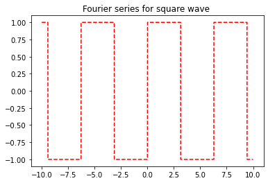
Figure above:

\[n(t) = -1 \quad ; \quad -\pi < t < 0\]

\[n(t) = 1 \quad ; \quad 0< t < \pi\]

## Solving Fourier Series in Python
t = sym.symbols('t')

x = sym.Piecewise((-1, t<0), (1, t>0))
series = sym.fourier_series(x, (t, -pi, pi))
series.truncate(5)

\[\displaystyle \frac{4 \sin{\left(t \right)}}{\pi} + \frac{4 \sin{\left(3 t \right)}}{3 \pi} + \frac{4 \sin{\left(5 t \right)}}{5 \pi} + \frac{4 \sin{\left(7 t \right)}}{7 \pi} + \frac{4 \sin{\left(9 t \right)}}{9 \pi}\]

The series are truncated at \(10\) components, due to Fourier series being infinite. Adding more components will make the plot look more similar to the box plot above.

Note that we know the box plot above is an odd function, hence we can assume the Fourier series are made up solely of sine functions, thus the \(b_m\) term is zero. If the function is even, we can expect only cosine functions, thus the \(a_n\) term is zero.

sym.plot(series.truncate(10), (t, -pi, pi))

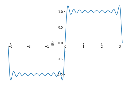
<sympy.plotting.plot.Plot at 0x7fa0dd7051c0>

Fourier transform

A fourier tranform changes the domain of a function from time to frequency. Any function can be composed of infinite series like sines and cosines. For example, in the plot above, Fourier series are used to make a box plot out of sine functions.

In the plot above, the series where truncated at \(10\) components. In the gif below is shown what happens if more and more components are added.

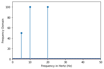
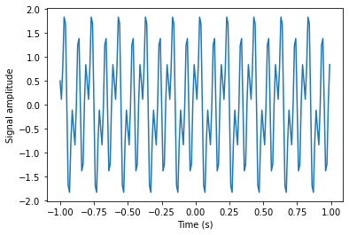
It can be seen that each component is a new function with a certain amplitude and period. These variables of each component can be displayed on a frequency spectrum. Decomposing the amplitudes of the components and the period can be done using a fourier transform. In Python, a ‘Fast Fourier Transform’ can be performed of which a frequency spectrum can be made.

f = 10  # frequency

t = np.linspace(-1, 1, 200, endpoint=False)
x = np.sin(f * 2 * np.pi * t) - np.sin(f * 4 * np.pi * t) + 0.5*np.cos(f * np.pi * t)

fig, ax = plt.subplots()
ax.plot(t, x)
ax.set_xlabel('Time (s)')
ax.set_ylabel('Signal amplitude');

X = fftpack.fft(x)
freqs = fftpack.fftfreq(len(x)) * 100 # 100 is sampling rate

fig, ax = plt.subplots()

ax.stem(freqs, np.abs(X))
ax.set_xlim(0, 50)
ax.set_ylim(0, 110)
ax.set_xlabel('Frequency in Hertz (Hz)')
ax.set_ylabel('Frequency Domain')

Text(0, 0.5, 'Frequency Domain')