Electricity and magnetism

Gravity, Magnetism, and Orbital Dynamics

This notebook will cover the basic principles, concepts and quantities surrounding the electric and magnetic fields. Electromagnetism is at the forefront of physics and engineering and is thus vital for any aspiring physicists and engineers to have a deep understanding of these concepts.

Coulomb’s law and the electric field

A stationary charge \(q_1\) at position \(\mathbf{r_1}\) produces a force on a charge \(q_2\) at \(\mathbf{r_2}\). Coulomb’s law describes this electrical interaction between two electrically charged particles in terms of the forces they exert on each other. This is given by

\[\mathbf{F_{12}} = \frac{q_1 q_2}{4{\pi}{\epsilon_0}{r_{12}^3}} \mathbf{r_{12}}\]

where \(\mathbf{r_{12}} ≡ r_2 − r_1\) and \(r_{12} = \mathbf{\left|r_{12}\right|}\).

The electric field, \(\mathbf{E(r)}\), of a charge illustartes how the electric force exerted by the charge on another charge varies with space. The field at a point \( \mathbf{r}\) due to a charge, \(q_1\) that has always been at \( \mathbf{r_1}\) is defined as

\[\mathbf{E(r)} = \frac{q_1}{4{\pi}{\epsilon_0}{\mathbf{\left|r - r_1\right|}^3}}\mathbf{\left[r - r_1\right]}\]

Now place a charge, \(q_2\), in the field. Using the 2 above definition we can see that the force exerted on \(q_2\) is related to the electric field by

\[\mathbf{F_{12}} = q_2 \mathbf{E(r)}\]

For a system containing \(n\) charges we can use the principle of superposition to show that the electric field of the system is

\[\mathbf{E} = \sum^{n}_{i = 1} \mathbf{E}_i\]

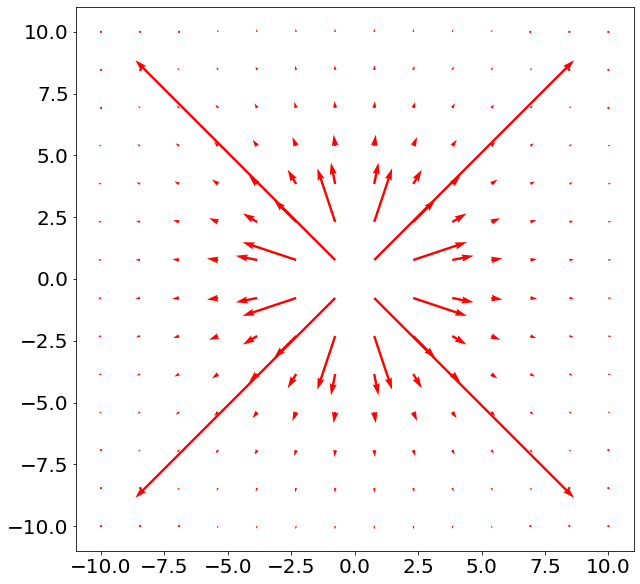
Below, the electric field, due to a positive point change at the origin, is plotted. The length of the arrows is an indication of the strength of the electric field at that point.

import numpy as np
import scipy as sp
import matplotlib.pyplot as plt

params = {
   'axes.labelsize': 20,
   'font.size': 20,
   'figure.figsize': [10, 10]
   } 
plt.rcParams.update(params)

def E(x,y):
    q= 1 #Charge in coulombs
    r1 = sp.array([0,0]) #Charge set at origin
    e0= 8.85*10**(-12) #permetivity of free space
    mag= (q / (4 * sp.pi* e0)) * (1 / ((x - r1[0])**2+ (y - r1[1])**2)) #Magnitude of Electric Field Strength
    ex= mag * ( np.sin(np.arctan2(x,y)))
    ey= mag * ( np.cos(np.arctan2(x,y)))
    
    return (ex,ey)

x=sp.linspace (-10,10,14)
y=sp.linspace (-10,10,14)

x,y=sp.meshgrid(x,y)

ex,ey=E(x,y)
plt.quiver(x,y,ex,ey, scale = 15000000000, color="red")
plt.show()

Electric potential

Consider a charge \(q\) in the electric field of another charge \(Q\). The charge \(q\) experiences a force, \(\mathbf{F}_Q\), due to the electric field. Now consider moving \(q\) from \(A \rightarrow B\) at constant speed. A force, \(\mathbf{F}_{ext}\) must be applied to match \(\mathbf{F}_Q\).Thus, in moving the charge the external force does work. Moving at constant speed

\[\mathbf{F}_{ext} + \mathbf{F}_Q = 0\]

and thus the work done by \(\mathbf{F}_{ext}\) on \(q\) is

\[dW = \mathbf{F}_{ext} \cdot d\boldsymbol{l} = - \mathbf{F}_{Q} \cdot d\boldsymbol{l}\]

Thus, the total work done by \(\mathbf{F}_{ext}\) is found by integrating from A to B

\[W = \int_{A}^{B} \mathbf{F}_{ext} \cdot d\boldsymbol{l} = - \int_{A}^{B} \mathbf{F}_{Q} \cdot d\boldsymbol{l}\]

The work done, \(W\), is equal to the change in potential energy, \(∆U\), and so

\[∆U = - \mathbf{F}_{Q} \cdot d\boldsymbol{l}\]

Using Coulombs law and carrying out the integration we find

\[∆U_{AB} = \frac{q Q}{4{\pi}{\epsilon_0}}\left(\frac{1}{r_B} - \frac{1}{r_A}\right)\]

and so the change in potential energy depends only on the radial seperation, r. Thus, \(∆U_{AB}\) is path independent, meaning that the shape of the path does not matter on the change of potential energy.

Potential difference

The potential difference between \(A\) and \(B\) is \(∆V_{AB}\) where

\[∆V_{AB} = \frac{∆U_{AB}}{q} = - \int_{A}^{B} \mathbf{E} \cdot d\boldsymbol{l}\]

\(∆V_{AB}\) is also path independent, and does not depend on \(q\) with an SI unit of \(JC^{−1}\). By choosing \(V = 0\) as \(r \rightarrow \infty\), we define the electric potential, \(V\), at \(P\) as the external work needed to bring a charge of \(+1 C\) at constant speed from \(r = ∞ \,(V = 0)\) to \(P\):

\[ V = - \int_{\infty}^{P} \mathbf{E} \cdot d\boldsymbol{l}\]

Key facts about \(V\): it is the potential energy / unit positive charge; it is a scalar field; and the superposition principle applies. With no external forces applied, positive charges move to lower potentials and negative charges move to higher potentials. For a point charge \(Q\), the potential \(V\) at \(r\) from \(Q\) is:

\[V = \frac{Q}{4{\pi}{\epsilon_0}r}\]

Magnetic flux

The magnetic field is represented by the letter \(\mathbf{B}\). Similarly to the electric field, \(\mathbf{B}\) is a vector field and has units of Tesla, \(T\). An important quantity is the magnetic flux, \(\mathbf{\Phi}\), defined as

\[\mathbf{\Phi} = \iint_{\mathbf{S}}^{} \mathbf{B} \cdot d\mathbf{S}\]

where \(\mathbf{S}\) is the vector pointing out of the surface under question. Thus, \(\mathbf{\Phi}\) is the magnetic flux through a surface and has units of Weber, \(Wb\) (\(Tm^2\)).

Lorentz force

The Lorentz force describes the force experienced by a charged object with charge \(q\) inside an electric and a magnetic field and is given by

\[\mathbf{F} = q(\mathbf{E} + \mathbf{v} \times \mathbf{B})\]

where \(\mathbf{v}\) is the velocity of the charged object. Assuming no electric field and a constant magnetic field, the particle will experience a perpendicular force to its motion where \(\mathbf{F} = \mathbf{F(v)}\). Thus \(\mathbf{B}\) is also a conservative quantity.

Magnetic dipole moment

Wires carrying a current have moving charges and thus current-carrying wires in a magnetic field can experience a force

\[\mathbf{F} = \int_{0}^{L} nqv \,d\boldsymbol{l} \times \mathbf{B}\]

where \(n\) is the charge density (\(m^{-1}\)). Current often flows in closed loops. Thus we define a new vector quantity, the magnetic dipole moment, \(\boldsymbol{\mu}\):

\[\boldsymbol{\mu} = I \mathbf{A}\]

where current \(I\) flows in a loop of area \(A\). \(\mathbf{A}\) is a vector based on the right hand rule on current. A magnetic field will exert a torque, \(\mathbf{\Gamma}\), on a current loop

\[\mathbf{\Gamma} = \boldsymbol{\mu} \times \mathbf{B}\]

Thus, magnetic fields exerts a torque on magnetic dipoles.