Data Structures
Contents
Data Structures#
Data structures allow us to speed up our algorithms often by many orders of magnitude. They arrange the data in a way that is suitable for the problem and usually simplify the workings of the algorithm. In this notebook, we will implement some of the most popular data structures in computer science:
Array#
Arrays are lists of objects. In some programming languages, arrays are objects of fixed length and have a type (e.g. list of 10 integers). In Python, are implemented using lists, which provide a little more flexibility by hosting multiple types and variable length. Arrays/lists support the following operation in complexity:
Set item (at index i smaller than the length): \(O(1)\)
Get item: \(O(1)\)
Deletion is no really supported as we assume that the array is of fixed length, for Python lists it is \(O(n)\).
Arrays are used in many programming problems where collections of data show up.
arr = [1,2,3]
# constant
arr[2] = 4
# constant
print(arr[1])
2
Stack#
A stack is a structure that follows that LIFO (last in, first out) rule. Elements can be pushed on top of the stack or popped of it. Those are the only two operations that this structure supports:
class Stack:
    def __init__(self):
        self.contents = []
    def pop(self):
        if len(self.contents):
            temp = self.contents[-1]
            self.contents = self.contents[:-1]
            return temp
        else:
            print("ERROR: Stack is empty")
    def push(self, elem):
        self.contents.append(elem)

st = Stack()
st.push(1)
print(st.pop())
st.pop()

# Python lists also support these operations, push is called append!
l = [1,2]
print(l.pop())
l.append(3)
print(l)
1
ERROR: Stack is empty
2
[1, 3]
Operations/complexity:
push: \(O(1)\)
pop: \(O(1)\)
One of popular problems utilizing stacks is checking whether an expression has balanced brackets. Let us limit ourselves to expressions consisting of [{,},(,)]. We will push the opening brackets on the stack and pop them when the closing bracket is approached. Of course, the types of brackets must match:
def checkIfValidBracketing(expr):
    # our stack :)
    st = []
    for i in expr:
        # not a bracket
        if i not in ["{","}","(",")"]:
            continue
        # push the opening bracket on the stack
        elif i in ["{","("]:
            st.append(i)
        # check when closing bracket approached
        elif i in ["}",")"]:
            try:
                temp = st.pop()
                if (i == "}" and temp == "{") or (i == ")" and temp == "("):
                    continue
                # invalid bracketing
                else:
                    return False
            except IndexError:
                return False
    return not len(st)

# Basic testing
print("{}()",checkIfValidBracketing("{}()"))
print("{(",checkIfValidBracketing("{("))
print("({()})",checkIfValidBracketing("({()})"))
print(")",checkIfValidBracketing(")"))
print("",checkIfValidBracketing(""))
{}() True
{( False
({()}) True
) False
 True
The following algorithm has \(O(n)\) time and space complexity.
Linked list#
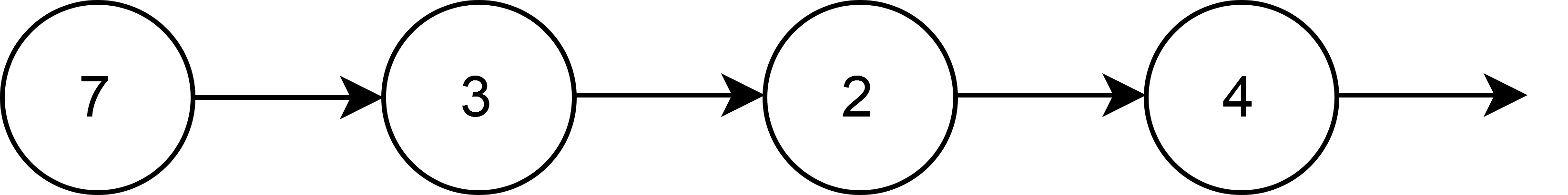
Linked lists are the simplest node-based structures. They are inherently recursive. A linked list consists of a head pointing to the next which itself is a linked list. The base case is an empty list:
A simple implementation would be:
class Node:
    def __init__(self,val):
        self.val = val
        self.next = None

class LinkedList:
    def __init__(self):
        self.head = None
    # insert at a position index
    # false is index out of range, true otherwise
    def insert(self,x, index):
        assert index >= 0
        newNode = Node(x)
        if not index:
            newNode.next = self.head
            self.head = newNode
            return True
        else:
            curr = self.head
            for _ in range(index-1):
                if curr is None:
                    return False
                curr = curr.next
            if curr is None:
                return False
            newNode.next = curr.next
            curr.next = newNode
            return True

    # remove item at index position
    # return true if the element was actually removed,
    # false otherwise
    def remove(self,index):
        assert index >= 0
        # Removing head
        if not index:
            if self.head is not None:
                self.head = self.head.next
                return True
            else:
                return False
        # index > 0
        else:
            curr = self.head
            for _ in range(index-1):
                if curr is None:
                    return False
                curr = curr.next
            if curr is None:
                return False
            else:
                if curr.next is None:
                    return False
                else:
                    curr.next = curr.next.next
                    return True

    # returns true if x in the list, false otherwise
    def search(self,x):
        curr = self.head
        while curr is not None:
            if curr.val == x:
                return True
            curr = curr.next
        return False

    # for testing and nice representation
    def __str__(self):
        res = ""
        curr = self.head
        while curr is not None:
            res += str(curr.val) + "->"
            curr = curr.next
        return res


ll = LinkedList()
print(ll)
print(ll.insert(0,0))
print(ll)
print(ll.insert(1,1))
print(ll)
print(ll.insert(2,1))
print(ll)
print(ll.remove(2))
print(ll)
print(ll.search(2))
print(ll.remove(0))
print(ll)
print(ll.search(0))
print(ll.remove(0))
print(ll.remove(0))
True
0->
True
0->1->
True
0->2->1->
True
0->2->
True
True
2->
False
True
False
All of these operations (insert,remove,search) take \(O(n)\) which is usually not optimal. There are numerous versions of linked lists e.g. doubly linked list which has nodes that point both to the previous and next nodes. Linked lists are often used to implement other data structures such as queues.
Queue#
Ques are similar to stacks but utilize the FIFO (first in, first out) rule. Basic ques support enqueue and dequeue operations. A linked list implementation would be:
class Node:
    def __init__(self, item):
        self.item = item
        self.next = None
        self.previous = None

class Queue:
    def __init__(self):
        self.length = 0
        self.head = None
        self.tail = None

    def enqueue(self, x):
        newNode = Node(x)
        if self.head == None:
            self.head = self.tail = newNode
        else:
            self.tail.next = newNode
            newNode.previous = self.tail
            self.tail = newNode
        self.length += 1

    def dequeue(self):
        if not self.length:
            return None
        item = self.head.item
        self.head = self.head.next
        self.length -= 1
        if self.length == 0:
            self.tail = None
        return item

    def __str__(self):
        res = ""
        curr = self.head
        while curr is not None:
            res += str(curr.item) + "->"
            curr = curr.next
        return res

queue = Queue()
print(queue)
queue.enqueue(1)
queue.enqueue(2)
queue.enqueue(3)
print(queue)
print(queue.dequeue())
print(queue)
print(queue.dequeue())
print(queue)
print(queue.dequeue())
print(queue)
print(queue.dequeue())
1->2->3->
1
2->3->
2
3->
3

None
With this implementation enqueue and dequeue are \(O(1)\). Queues are used in numerous problems, such as graph traversals (BFS).
Binary search tree (BST)#
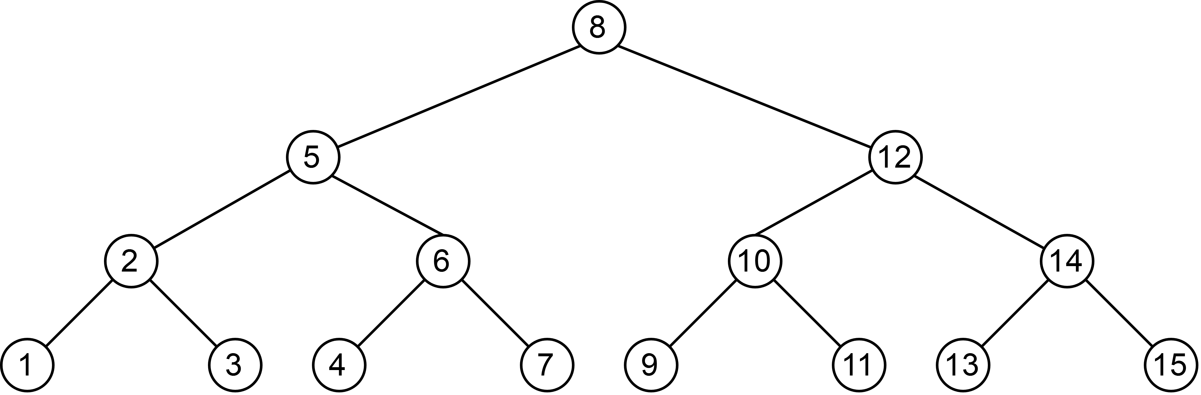
Binary tree is another node-based structure also recursive in nature. The tree consists of a root which points to at most two children which are also binary trees. Binary search trees are a type of binary trees which have the property that the key of the left child is no greater than the root key. Right child’s key is greater than the root key. An example binary search tree is as follows:
An example implementation for BST with integers is as follows:
# implemented as a set, will not contain duplicates
class BST:
    def __init__(self,val=None):
        self.val = val
        self.left = None
        self.right = None

    # true if the insert changes the BST
    def insert(self,x):
        if self.val is None:
            self.val = x
            return True
        # already in the set
        elif self.val == x:
            return False
        elif self.val > x:
            if self.left is None:
                self.left = BST(x)
                return True
            else:
                return self.left.insert(x)
        else:
            if self.right is None:
                self.right = BST(x)
                return True
            else:
                return self.right.insert(x)

    # seach for x in BST
    def search(self,x):
        if self.val is None:
            return False
        elif self.val == x:
            return True
        elif self.val > x:
            if self.left is None:
                return False
            else:
                return self.left.search(x)
        else:
            if self.right is None:
                return False
            else:
                return self.right.search(x)
Node removal is a bit more involved and will not be covered. All basic operations can be done in \(O(\log(n))\). BST can be used to speed up many problems that require repetitive searching of the data. Consider the following problem:
Numbers smaller than the given number in an array You are given an array of integers. You should provide a data structure which should return the number of elements smaller than any chosen element in the array.
We will solve the question by constructing a BST out of the array that will store the the number of nodes to the left of the node (its rank):
class newNode:
    def __init__(self, data):
        self.data = data
        self.left = self.right = None
        self.leftSize = 0

# Inserting a new Node.
def insert(root, data):
    if root is None:
        return newNode(data)

    # Updating size of left subtree.
    if data <= root.data:
        root.left = insert(root.left, data)
        root.leftSize += 1
    else:
        root.right = insert(root.right, data)
    return root

# Function to get Rank of a Node x.
def getRank(root, x):
    if root.data == x:
        return root.leftSize
    if x < root.data:
        if root.left is None:
            return -1
        else:
            return getRank(root.left, x)
    else:
        if root.right is None:
            return -1
        else:
            rightSize = getRank(root.right, x)
            if rightSize == -1:
                # x not found in right sub tree, i.e. not found in stream
                return -1
            else:
                return root.leftSize + 1 + rightSize
arr = [5, 1, 4, 4, 5, 9, 7, 13, 3]
root = None
for i in range(len(arr)):
    root = insert(root, arr[i])
print(getRank(root, 4))
print(getRank(root, 13))
print(getRank(root, 8))
3
8
-1
This algorithm will work in \(O(\log(n))\) time on average. However, of the array was initially sorted the formed tree will be degenerate (it will form a linked list). We will learn how to solve such cases in AVL trees.
Heap#
Heaps (especially binary heaps) are tree-like structures that have two properties:
They are a complete tree (all levels of the tree are filled except possibly the last level).
It is either a min-heap or a max-heap. In the first case, the root is smaller or equal to its children. The opposite is true for the max heap.
Let us implement a min-heap storing integers. It will support taking the top element (which is the minimum) as well as inserting new elements. Interestingly, we will implement it using a Python list. It is an important fact to spot that a parent of an element at index i is at index i//2.
# utility functions
def swap(arr, x, y):
    temp = arr[x]
    arr[x] = arr[y]
    arr[y] = temp

class MinHeap:
    def __init__(self):
        self.contents = []
        self.size = 0

    # utility function
    def heapifyUp(self, i):
        while i // 2 > 0:
            if self.contents[i-1] < self.contents[i // 2 - 1]:
                swap(self.contents,  i-1, i // 2 - 1)
            i //= 2

    def insert(self,val):
        self.size += 1
        self.contents.append(val)
        self.heapifyUp(self.size)

    def heapifyDown(self,i):
        while (2 * i + 1) < self.size:
            mc = self.minChild(i)
            if self.contents[i] > self.contents[mc]:
                swap(self.contents, i, mc)
            i = mc

    def minChild(self, i):
        if 2 * i + 2 >= self.size:
            return 2 * i + 1
        else:
            if self.contents[2 * i + 1] < self.contents[2 * i + 2]:
                return 2 * i + 1
            else:
                return 2 * i + 2

    def getMin(self):
        assert self.size > 0
        self.size -= 1
        res = self.contents[0]
        swap(self.contents,0, self.size)
        self.contents.pop()
        self.heapifyDown(0)
        return res

#Heapsort -  a O(nlog(n)) sorting algorithm.

arr = [1,3,2,6,8,3,4,5,6,7,2,3,8]
heap = MinHeap()

for j in range(len(arr)):
    heap.insert(arr[j])

print(heap.contents)
arr = []
while heap.size:
    arr.append(heap.getMin())
print(arr)
[1, 2, 2, 5, 3, 3, 4, 6, 6, 8, 7, 3, 8]
[1, 2, 2, 3, 3, 3, 4, 5, 6, 6, 7, 8, 8]
Heaps have many, many uses. One of such is HeapSort - a \(O(n\log(n))\) sorting algorithm (see above). Heaps are also used in priority queues - queues which have the elements sorted by some priority such as objects sorted by their value.
AVL Tree#
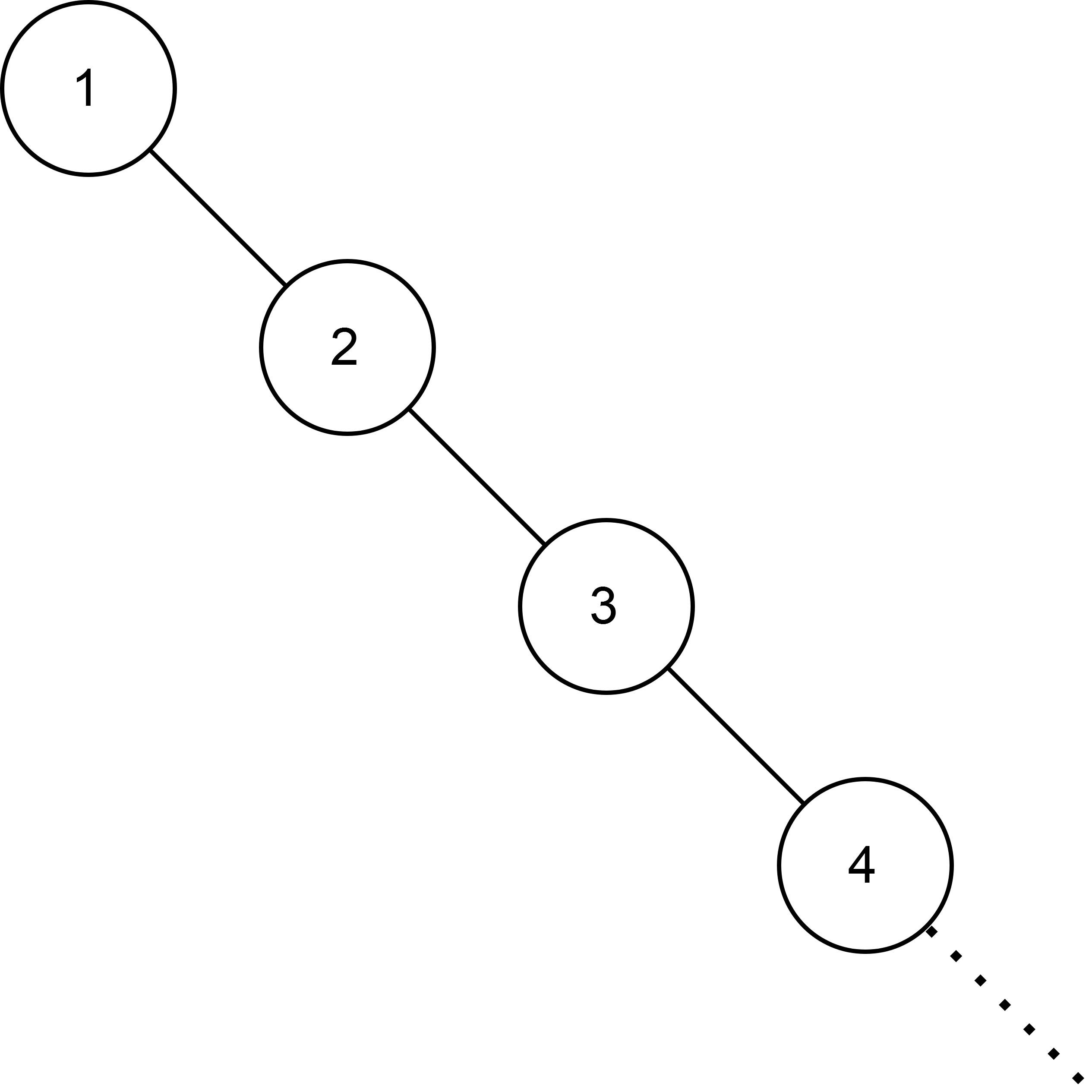
Consider the case we insert a sorted list into a regular BST. We would end up with the following structure:
This tree is degenerate. Search operations are \(O(n)\) which is too slow for many implementations. To counter the degeneration we can utilize self-balancing binary trees such as the AVL tree (named after Adelson-Velsky and Landis). This type of tree holds the invariant that for each node the difference in heights between left and right subtree is at most 1. Let us see how it is achieved.
AVL insertion#
The first stage of insertion is the same as in BST, we recurse down the tree until we find an appropriate spot for the new value.
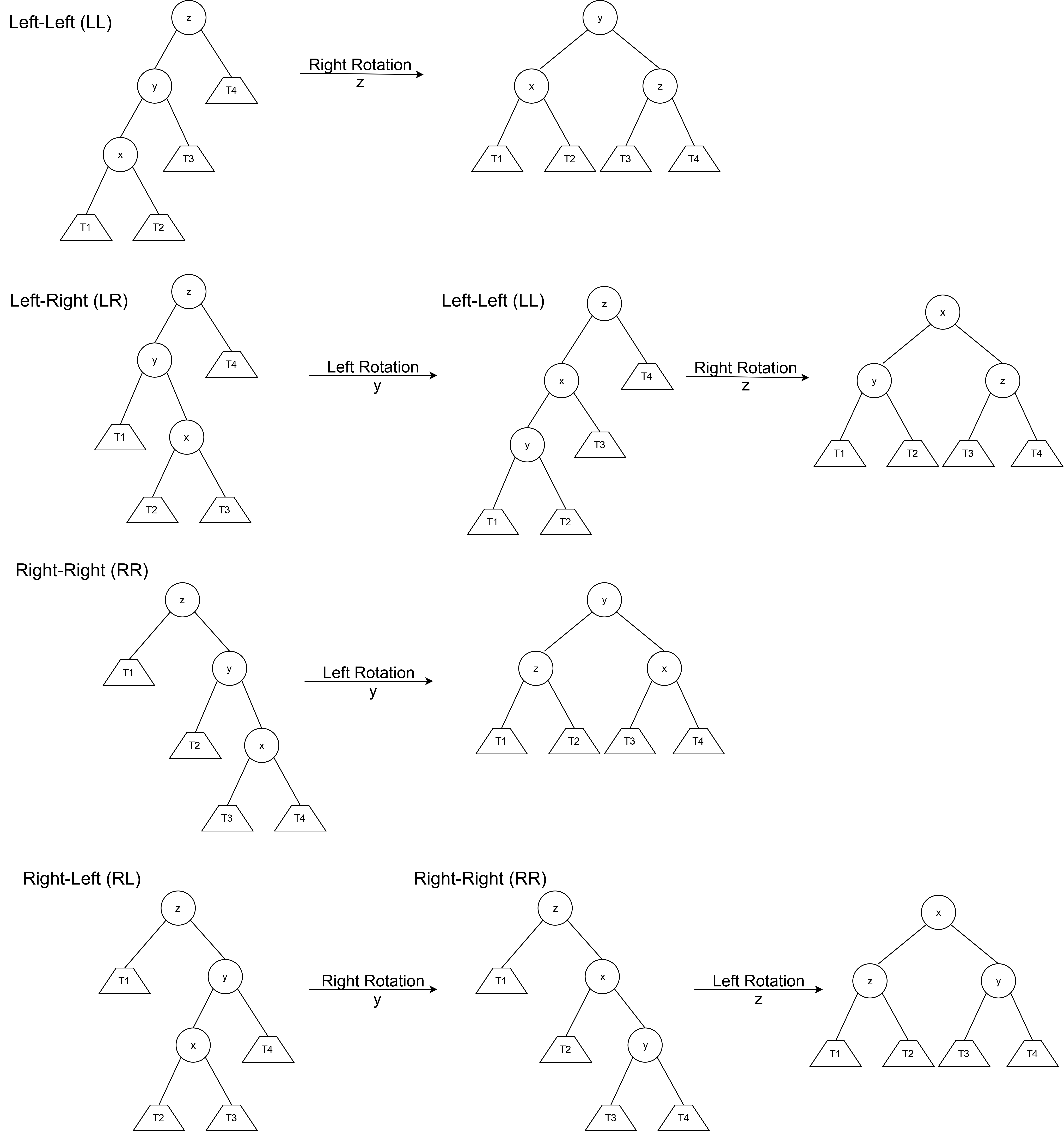
Each node in the AVL tree has a height (the distance between the node and the farthest leaf node in the children). We check if the difference in heights of children exceeds 1 in absolute value. If so, the tree is imbalanced. Such violation can occur in four possible ways (see the diagram below). We will use node rotations to solve the problem:
The implementation of the AVL tree is presented below, please take a while to digest it. The topic is not trivial. Also, have a look at the comparison between the BST and AVL in the degenerate case:
import time
# we will support only insertions and deletions
class AVLNode:
    # has to be initialised with a root value
    def __init__(self,val):
        self.val = val
        self.left = None
        self.right = None
        self.height = 0

    # searching is the same as in regural BST
    def search(self,val):
        if val == self.val:
            return True
        elif val < self.val:
            if self.left is not None:
                return self.left.search(val)
            else:
                return False
        else:
            if self.right is not None:
                return self.right.search(val)
            else:
                return False

    def insert(self, root, val):
        # Normal BST insert
        if not root:
            return AVLNode(val)
        elif root.val  == val:
            return root
        elif val < root.val:
            root.left = self.insert(root.left,val)
        else:
            root.right = self.insert(root.right,val)

        # update the height of the root
        root.height = 1 + max(getHeight(root.left), getHeight(root.right))
        # get the balance factor
        balance = getBalance(root)
        # consider 4 cases
        # LL
        if balance > 1 and val < root.left.val:
            return rotateRight(root)
        # RR
        if balance < -1 and val > root.right.val:
            return rotateLeft(root)
        # LR
        if balance > 1 and val > root.left.val:
            root.left = rotateLeft(root.left)
            return rotateRight(root)
        # RL
        if balance < -1 and val < root.right:
            root.right = rotateRight(root.right)
            return rotateLeft(root)
        return root

# UTILITY FUNCTIONS
#_____________________________________________
# how is the tree unbalanced?
def getBalance(node):
    if not node:
        return 0
    else:
        return getHeight(node.left) - getHeight(node.right)

# get height of a node
def getHeight(node):
    if not node:
        return 0
    else:
        return node.height

def rotateRight(node):
    # do the rewiring
    z = node
    y = z.left
    T3 = y.right

    y.right = z
    z.left = T3

    # update heights
    z.height = 1 + max(getHeight(z.left),
                       getHeight(z.right))
    y.height = 1 + max(getHeight(y.left),
                       getHeight(y.right))
    return y

def rotateLeft(node):
    # do the rewiring
    z = node
    y = z.right
    T2 = y.left

    y.left = z
    z.right = T2

    # update heights
    z.height = 1 + max(getHeight(z.left),
                       getHeight(z.right))
    y.height = 1 + max(getHeight(y.left),
                       getHeight(y.right))
    return y
#_____________________________________________

# Change the code below according to your preference
arr = list(range(1000))

t = time.time()
bst = BST(0)
avl = AVLNode(0)

for i in arr:
    bst.insert(i)
    bst.search(i)

print("BST time:",time.time() - t)
t = time.time()

for i in arr:
    avl = avl.insert(avl, i)
    avl.search(i)

print("AVL time:", time.time() - t)
print("Height of the AVL Tree: " + str(avl.height))
BST time: 0.538590669631958
AVL time: 0.014953136444091797
Height of the AVL Tree: 10
Hash Table#
In simple terms, a hash table is identical to Python dict dictionaries. They allow us to retrieve objects (given their key) in \(O(1)\) time on average. They also allow for constant time insertion and deletion. Wait, what? Does it mean that they are ultimately the fastest data structures? - as you can probably guess it is not that simple. It will become clear as we will implement a simple hash table:
A hash table is similar to an array. It has some fixed capacity which can be changed (not in constant time). The elements are indexed by the key values. For the hash table to work, the elements need to be indexed by integer values. A special function, called the hash function transforms the key values to integers. The basic utilities needed by a hash table are shown in the class below:
class HashTable:
    def __init__(self,size = 8):
        pass

    #Insert a new key-value pair or overwrite an existing one
    def insert(self,key, value):
        pass

    # Overload the [] index access
    def __setitem__(self,key,value):
        return self.insert(key,value)

    # Retreive the value given the key
    def get(self, key):
        pass

   # Overload the [] index access
    def __getitem__(self,key):
        return self.get(key)

    # Computes the hash position
    def _hash(self,key):
        pass
Hash function#
First, we will choose a hash function which will map keys to particular positions in the array. There are multiple ways of approaching this problem. Two simple ones include:
The mod method In this case, we take the remainder of dividing the key by the table-size:
h(key) = key % table_size
This is a very fast hash function. However, many keys can have the same hash which results in collisions (e.g. 64 % 8 and 8 % 8 are both 0). We discuss those below.
The multiplication method First we multiply the key by
0 < c < 1and take the fractional part ofk * cwhich isk * c - floor(k * c). This method leads to fewer overlaps and therefore we will use it in our implementation. Some values ofcwork better statistically.c ~ (sqrt (5) – 1) / 2is likely to work well.
h(key) = floor(table_size * (key * c - floor(key * c)))
Both of these functions can lead to inefficient hash tables with operations with \(O(n)\) worst-case time. There are more advanced methods which solve this problem, which you are free to research here.
Overlaps#
When two different keys are mapped to the same hash value we are dealing with an overlap. The way our implementation will tackle this problem is by chaining. Each entry in the table will be a linked list-like object. In case of an overlap, we will append at the end of such a list. Of course, in the case when all elements collide we will one big linked-list object. The role of our hash function is to minimise the probability of this happening.
Doubling#
Let n denote the number of elements in the hash table. The load factor is defined as n / table_size. As our table becomes more filled more cells (on average) become linked lists. To counter this effect we will double the size of the table when the load factor reaches a certain value (in our case \(1\)). We will not support deletion therefore shrinking is not essential.
With all this knowledge let us provide an implementation:
import math, random
# We will support string keys
# it could be easily translated to integer keys
# the table will be a 2d array of tuples (key,value)
class HashTable:
    def __init__(self,size = 8):
        self.contents = []
        self.size = size
        self.load = 0
        for _ in range(self.size):
            self.contents.append([])

    #Insert a new key-value pair or overwrite an existing one
    def insert(self,key, value):
        elem = (key, value)
        # calculate the hash value
        hashVal = self._hash(key)
        # insert the element (chaining)
        # check in elem already in
        if elem not in self.contents[hashVal]:
            self.contents[hashVal].append(elem)
            # increase the load
            self.load += 1
        # doubling
        if self.load / self.size > 1:
            # double the size
            self.size *= 2
            # make new contents table
            newContents = []
            for _ in range(self.size):
                newContents.append([])
            # insert the old elements
            for i in self.contents:
                for j in i:
                    hashVal = self._hash(j[0])
                    # insert the element (chaining)
                    newContents[hashVal].append(j)
            self.contents = newContents

    # Overload the [] index access
    def __setitem__(self,key,value):
        return self.insert(key,value)

    # Retreive the value given the key
    def get(self, key):
        hashVal = self._hash(key)
        for i in self.contents[hashVal]:
            if i[0] == key:
                return i[1]
        print("Key has no value associated")

   # Overload the [] index access
    def __getitem__(self,key):
        return self.get(key)

    # Computes the hash position
    def _hash(self,key):
        k = sum(ord(c) for c in key)
        c = (math.sqrt(5) - 1) / 2
        return min(math.floor(self.size * (k * c - math.floor(k * c))),self.size - 1)

# Testing out
ht = HashTable()
for _ in range(16):
    temp = ''
    for i in range(random.randint(1,5)):
        temp += chr(random.randint(ord('a'),ord('z')))
    ht[temp] = random.randint(0,17)
    print(ht[temp])
print(ht.contents)
4
7
4
0
6
4
3
1
11
8
7
3
17
8
5
5
[[], [], [('lemo', 3), ('emz', 5)], [], [('ps', 0)], [('sdens', 4), ('jbzni', 3)], [('jcpgq', 17)], [('zjb', 7)], [('w', 4), ('cbl', 8)], [], [], [], [('xsfj', 5)], [('po', 7), ('sazku', 4), ('udl', 1), ('vv', 8)], [('i', 11)], [('n', 6)]]
References#
Cormen, Leiserson, Rivest, Stein, “Introduction to Algorithms”, Third Edition, MIT Press, 2009
GeeksforGeeks, Rank Elements in an Integer Stream (BST)
Pythonds, Binary Heap Implementation
GeeksforGeeks, AVL Insertion
Sebastian Raschka, Github, Implementing a Simple Hash Table
GeeksforGeeks, Implementation of Hashing with Chaining in Python