Dynamic Programming
Contents
Dynamic Programming#
Dynamic algorithms are a family of programs which (broadly speaking) share the feature of utilising solutions to subproblems in coming up with an optimal solution. We will discuss the conditions which problems need to satisfy to be solved dynamically but let us first have a look at some basic examples. The concept is quite challenging to digest, so there are many examples in this section.
Simple Examples#
Dynamic Fibonacci If you have read the section about recursion you probably know that the basic implementation for generating Fibonacci numbers is very inefficient (\(O(2^n)\)!). Now, as we generate the next numbers in the Fibonacci sequence, we will remember them for further use. The trade-off between memory and time is dramatic in this case. Compare the two versions of the function:
# For comparing the running times
import time

# Inefficient
def fib(n):
    assert n >= 0
    if n < 2:
        return 1
    else:
        return fib(n-1) + fib(n-2)

# Dynamic version
def dynamicFib(n):
    assert n >= 0
    #prepare a table for memoizing
    prevFib = 1
    prevPrevFib = 1
    temp = 0

    #build up on your previous results
    for i in range(2,n+1):
        temp = prevFib + prevPrevFib
        prevPrevFib = prevFib
        prevFib = temp
    return prevFib

start = time.time()
print(fib(32))
end = time.time()
print("Time for brute:" + str(end - start))

start = time.time()
print(dynamicFib(32))
end = time.time()
print("Time for dynamic:" + str(end - start))
3524578
Time for brute:0.8238296508789062
3524578
Time for dynamic:0.0
The time difference is enormous! As you can probably spot, dynamicFib is \(O(n)\)! With the use of three integer variables (prevFib, prevPrevFib and temp) we brought exponential time complexity down to linear. How did it happen? Let us now depict the work done by fib(5) on a graph:
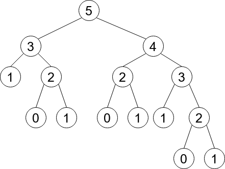
Wow! This is quite a tree! However, the worst feature is that many of the nodes are repeated (e.g. node \(2\) appears 3 times). These repeated results which are constantly recomputed bring us to the exponential complexity. Consider the dynamic solution graph:
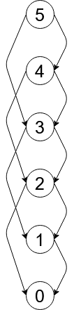
Now, the number of nodes grows linearly with \(n\). We have merged the subproblems to avoid redundancy.
Shortest Path on a Grid Dynamic programming is often used for optimisation problems. Consider a square grid with numbers from 0 to 9 in each square. An example would be:
+-+-+-+-+
|1|0|8|4|
+-+-+-+-+
|3|5|1|0|
+-+-+-+-+
|6|8|9|3|
+-+-+-+-+
|1|2|4|5|
+-+-+-+-+
It is allowed to move only down or right. What is the value of the minimum path from the upper-left corner to the lower-right corner?
The initial approach to the problem might be to check all the possible paths and return the minimal one. This is exponential and too slow. To come up with a faster approach we need to find subproblems.
Let us imagine that we have reached the lower-right corner (hurray!). We could get there from the tile above it and left of it. This might at first seem like a Divide and Conquer problem, but let us keep on looking for an overlap:
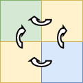
In the simplest case of four tiles, we can already see that the upper-left tile is considered twice. We should then leverage this repetition. This overlapping generalises for larger grids. In our algorithm, we will remember the optimal path to the tiles already visited and build on this knowledge:
# grid is a square matrix
def shortestPathDownRight(grid):
    # dictionary that will keep the optimal paths
    # to the already visited tiles
    table = {}
    # n - length of the side of the square
    n = len(grid)
    assert n == 0 or len(grid[0]) == n
    table[(0,0)] = grid[0][0]
    # top and most left column have trival optimal paths
    for i in range(1, n):
        table[(0,i)] = table[(0,i-1)] + grid[0][i]
        table[(i,0)] = table[(i-1,0)] + grid[i][0]
    # the dynamic magic
    for i in range(1,n):
        for j in range(1,n):
            table[(i,j)] = min(table[(i-1,j)],table[(i,j-1)]) + grid[i][j]

    return table[(n-1,n-1)]

grid = [[1,0,8,4],[3,5,1,0],[6,8,9,3],[1,2,4,5]]
print(shortestPathDownRight(grid))
15
What is the time complexity of this algorithm? Based on the nested loop we can deduce that it is \(O(n^2)\). Quite an improvement!
Space Complexity#
We usually do not concern ourselves with the amount of memory a program utilises. Dynamic programs are an exception to this rule. The amount of memory they use can be a limiting factor for some machines, so we need to take it into account. In the case of dynamicFib this was \(O(1)\) as we only needed to keep track of the last two Fibonacci numbers. In case of shortestPathDownRight we need to create a grid of size \(n \times n\), so \(O(n^2)\). The notion of space complexity is very similar to time complexity, so we will not discuss it in depth.
Cutting Rods We are given a rod of integer length \(n\) and a list of length
prices\(n\). The \(i\)th entry in the list corresponds to the profit we can get from selling the rod of length \(i\). How should we cut the rod so we maximise our profit? The key to our dynamic algorithm will be the observation that:
We cut the rod at position \(k\). Now we have a rod of lenght \(k\) and \(n-k\). Let us assume we know the maximum price for these two rods. Now we need to consider all the \(0 \leq k \leq \lfloor \frac{n}{2} \rfloor + 1\) (the problem is symmetric so computing for \(\frac{n}{2} \leq k\) would be redundant. For \(k=0\) we just take prices[n]. The cutting introduces subproblems which are smaller than the initial problem and they are overlapping! Let us put this into code:
# For comparing the running times
import time
# For testing
from random import randint

def dynamicCutRod(n,prices):
    # setting the initial values of variables
    assert n >= 0 and n == len(prices)
    # trival cases
    if n == 0:
        return 0
    if n == 1:
        return prices[0]

    # setting up needed variables
    table = {}
    currLen = 2
    table[0] = 0
    table[1] = prices[0]
    while currLen < n + 1:
        # no cuts for a given len
        table[currLen] = prices[currLen - 1]
        # considering all possible cuts for a give len
        for k in range(1,currLen//2 + 1):
            # take the maximal one
            if table[currLen] < table[k] + table[currLen - k]:
                table[currLen] = table[k] + table[currLen - k]
        currLen += 1
    return table[n]

# for testing purposes
def bruteForceRecursive(n,prices):
    assert n >=0
    if n == 0:
        return 0
    if n == 1:
        return prices[0]
    currLen = n
    res = prices[n-1]
    for k in range(1,n//2 + 1):
        res = max(res, bruteForceRecursive(k,prices) + bruteForceRecursive(n-k,prices))
    return res

# testing
for i in range(1, 11):
    prices = []
    for j in range(i):
        prices.append(randint(1,10))

    assert bruteForceRecursive(len(prices),prices) == dynamicCutRod(len(prices),prices)

# comparing times
prices = []
for i in range(20):
    prices.append(randint(1,10))

start = time.time()
print(bruteForceRecursive(len(prices),prices))
end = time.time()
print("Time for brute:" + str(end - start))

start = time.time()
print(dynamicCutRod(len(prices),prices))
end = time.time()
print("Time for dynamic:" + str(end - start))
66
Time for brute:1.457252025604248
66
Time for dynamic:0.0029768943786621094
Time complexity? For each \(0\leq i \leq n \) we need to consider \(i\) different cuts. This is the sum of arithmetic series so \(O(n^2)\). We memoize only the optimal solutions to subproblems, therefore space complexity is \(O(n)\).
Characteristic features of dynamic problems#
All problems which can be tackled with the use of Dynamic Programming (DP) have two main features:
Optimal substructure: In broad terms, that solution to the problem can be formulated in terms of independent subproblems. Then you choose a solution/combination of optimal solutions to subproblems and show that this choice leads to an optimal global solution. For example, for the
shortestPathproblem we choose between the optimal solution to the tile above and tile to the left. For the rod problem, we choose between all possible \(n\) cuts of a rod and assume we have solutions to the shorter rods.Overlapping subproblems: The subproblems which we split the main question into should repeat. Eliminating the need to recompute the subproblems (by memoising them) should speed up our algorithm. For example,
dynamicFibused two variables to keep the results of computing previous Fibonacci numbers.
Common approaches to DP#
There are two main schools of thought when it comes to solving DP algorithms:
Memoization is using the memory-time trade-off. It remembers the results to the subproblems in a dictionary
memoand recalls them when needed. If we have the result in memory, we take if from there, otherwise compute it.Bottom-up approach starts with the trivial cases of the problem and builds on them. I relies on the the fact that subproblems can be sorted. So we first compute the optimal cutting for a rod of length 1 and then length 2 and so on…
Both usually lead to the same time complexities.
Advanced Examples#
0-1 Knapsack The problem is about a backpack (knapsack) of an integer volume \(S\), we are given lists
spacesandvalswhich correspond to the size and value of the objects we might want to pack. The trick is to pack the objects of the highest accumulate value which fit into the backpack. We will consider prefixes of thesizeslist in order of length and put the intermediate results in a table. Compare the bottom-up and memoized approaches:
# For comparing the running times
import time
# For testing
from random import randint

# bottom up approach
def knapSack(wt, val, W, n):
    K = [[0 for x in range(W + 1)] for x in range(n + 1)]

    # Build table K[][] in bottom up manner
    for i in range(n + 1):
        for w in range(W + 1):
            if i == 0 or w == 0:
                K[i][w] = 0
            elif wt[i-1] <= w:
                K[i][w] = max(val[i-1] + K[i-1][w-wt[i-1]],  K[i-1][w])
            else:
                K[i][w] = K[i-1][w]

    return K[n][W]

# memoized
memo = {}
def knapSackMemo(wt,val, W, n):
    # base case
    if n == 0 or W == 0:
        memo[(n,W)] = 0
        return 0
    # check if memoized
    if (n,W) in memo:
        return memo[(n,W)]
    # if not, calcuate
    else:
        if wt[n-1] <= W:
            memo[(n,W)] = max(knapSackMemo(wt,val,W-wt[n-1],n-1)+val[n-1],
                              knapSackMemo(wt,val,W,n-1))
            return memo[(n,W)]
        else:
            memo[(n,W)] = knapSackMemo(wt,val,W,n-1)
            return memo[(n,W)]

# brute force for testing
def bruteForce(wt, val, W):
    res = 0
    # all combinations of the elements
    for i in range(2**len(wt)):
        sumSize = 0
        sumVal = 0
        for j in range(len(wt)):
            if (i >> j) & 1:
                sumSize += wt[j]
                sumVal += val[j]
            if sumSize > W:
                sumVal = 0
                break
        res = max(sumVal, res)
    return res

# testing
for _ in range(10):
    sizes = []
    vals = []
    S = randint(0,200)
    memo = {}
    for _ in range(13):
        sizes.append(randint(1,10))
        vals.append(randint(1,20))

    br = bruteForce(sizes,vals, S)
    btup  = knapSack(sizes,vals,S,len(sizes))
    mem = knapSackMemo(sizes,vals,S,len(sizes))

    assert btup == br and mem == br

start = time.time()
print(bruteForce(sizes,vals, S))
end = time.time()
print("Time for brute:" + str(end - start))

start = time.time()
print(knapSack(sizes,vals,S,len(sizes)))
end = time.time()
print("Time for bottom-up:" + str(end - start))

memo = {}
start = time.time()
print(knapSackMemo(sizes,vals,S,len(sizes)))
end = time.time()
print("Time for memoized:" + str(end - start))
135
Time for brute:0.019960880279541016
135
Time for bottom-up:0.00098419189453125
135
Time for memoized:0.0009658336639404297
In this case, the memoized approach is the fastest as it does not usually require to consider all (n,W) pairs. However, both bottom-up and memoized approach have space (and time) complexity of \(O(nS)\). The brute force has time complexity of \(O(2^n)\), where \(n\) is the length of the sizes list.
Scheduling With all the chaos that COVID caused universities are going fully remote. The head of your department asked the lecturers to send the timeslots in which they can do lectures. This is a list
timeslotswhich consist of pairs of integers - the start and end of the timeslot. If timeslots overlap, then we choose only one of them. Lectures can start at the same time the previous lecture finished. You aim to pick the subset oftimeslotswhich assures that the sum of teaching hours is maximum. Return the maximum number of hours.
The question is similar to the previous one. We are given a list of items (timeslots) and need to come up with an optimisation. The value of each subset is the sum of hours of its elements. To speed things up in later stages, we will sort the timeslots by the ending time. This is done in \(O(n\log(n))\). We will then consider the prefixes of the sorted array and memoize optimal results. memo[n] will store the maximum number of hours from the prefix of n length.
# For comparing the running times
import time
# For testing
from random import randint

# utility function to speed up the search
def binarySearch(timeslots,s,low,high):
    if low >= high:
        return low
    mid  = (low + high) //2
    if timeslots[mid][1] <= s:
        return binarySearch(timeslots, s, mid+1, high)
    else:
         return binarySearch(timeslots, s, low, mid)

# init memo
memo = {}
# assumes that timeslots array is sorted by ending time
def schedule(timeslots, n):
    # base case
    if n == 0:
        memo[0] = 0
        return 0
    # memoized case
    elif n in memo:
        return memo[n]
    # else calculate
    else:
        s,e = timeslots[n-1]
        # in log time
        ind = min(binarySearch(timeslots,s,0,len(timeslots)),n-1)
        memo[n] = max(schedule(timeslots,n-1), schedule(timeslots,ind) + (e - s))
        return memo[n]

# brute force for testing
def bruteForce(timeslots):
    res = 0
    # all combinations of the elements
    for i in range(2**len(timeslots)):
        sumHours = 0
        already_chosen = []
        for j in range(len(timeslots)):
            if (i >> j) & 1:
                s, e = timeslots[j]
                sumHours += e - s
                already_chosen.append(timeslots[j])
            # checking if a valid combination of timeslots
            for k in range(len(already_chosen)-1):
                if not (s >= already_chosen[k][1] or e <= already_chosen[k][0]):
                    sumHours = 0
                    break
        res = max(sumHours, res)
    return res

# testing
for _ in range(10):
    memo = {}
    timeslots = []
    for _ in range(12):
        s = randint(0,100)
        e = randint(s,100)
        timeslots.append((s,e))
    timeslots.sort(key = lambda slot: (slot[1],slot[0]))

    br = bruteForce(timeslots)
    mem = schedule(timeslots,len(timeslots))
    assert br == mem

start = time.time()
print(bruteForce(timeslots))
end = time.time()
print("Time for brute:" + str(end - start))

memo = {}
start = time.time()
print(schedule(timeslots,len(timeslots)))
end = time.time()
print("Time for memo:" + str(end - start))
82
Time for brute:0.14516472816467285
82
Time for memo:0.0010349750518798828
Time complexity of this solution is \(O(n\log(n))\). Why?
Exercises#
Tiling problem You are given a \(2 \times n\) board and \(2 \times 1\) tiles. Count the number of ways the tiles can be arranged (horizontally and vertically) on the board.
HINT: You have seen this algorithm before.
Answer
Consider the end of the board. There are two cases, we can either have to fill in a \(2 \times 2\) subboard or \(1 \times 2\) subboard. We assume that the rest of the board is already covered and this is the same problem but smaller. There are two ways of arranging tiles on the \(2 \times 2\) board and one way to do this on \(1 \times 2\) board. Watch out though! The case in which we place tiles vertically on the \(2 \times 2\) board covers some of the cases when we fill \(1 \times 2\). Therefore we should ignore it. The final formula is as follow:
That is Fibonacci numbers.
Maximum sum subarray You are given an array with \(1\) and \(-1\) elements only. Find the array of the maximum sum in \(O(n)\). Return this maximal sum. E.g. [-1,1,1,-1,1,1,1,-1] -> 4.
HINT: Consider the sums of prefixes of the array.
Answer
def maxSubarray(arr):
    assert len(arr) > 0
    sumPref = 0
    minSum = 0
    maxSum = 0
    for i in range(0,len(arr)):
        # current prefix sum
        sumPref = sumPref + arr[i]
        # keep track of the minimal sum (can be negative)
        minSum = min(minSum, sumPref)
        # take away the minSum, this will give max
        maxSum = max(maxSum, sumPref-minSum)
    return maxSum

print(maxSubarray([-1,1,1,-1,1,1,1,-1]))
Longest snake sequence You are given a grid of natural numbers. A snake is a sequence of numbers which goes down or to the right. The adjacent numbers in a snake differ by a maximum 1. Define a dynamic function which will return the length of the longest snake. E.g.
9, 6, 5, 2
8, 7, 6, 5
7, 3, 1, 6
1, 1, 1, 7
-> 7
Answer
def longestSnake(grid):
    #dictionary that will keep the optimal paths to the already visited tiles
    table = {}
    # n - length of the side of the square
    n = len(grid)
    assert n == 0 or len(grid[0]) == n
    table[(0,0)] = 1
    # top and most left column have trival optimal paths
    for i in range(1, n):
        table[(0,i)] = table[(0,i-1)] + 1 if abs(grid[0][i] - grid[0][i-1]) < 2 else 1
        table[(i,0)] = table[(i-1,0)] + 1 if abs(grid[i][0] - grid[i-1][0]) < 2 else 1
    # the dynamic magic
    for i in range(1,n):
        for j in range(1,n):
            table[(i,j)] = max(
                table[(i-1,j)] + 1 if abs(grid[i][j] - grid[i-1][j]) < 2 else 1,
                table[(i,j-1)] + 1 if abs(grid[i][j] - grid[i][j-1]) < 2 else 1)

    return max(table.values())

mat = [[9, 6, 5, 2],
       [8, 7, 6, 5],
       [7, 3, 1, 6],
       [1, 1, 1, 7]]

print(longestSnake(mat))
References#
Cormen, Leiserson, Rivest, Stein, “Introduction to Algorithms”, Third Edition, MIT Press, 2009
Prof. Erik Demaine, Prof. Srini Devadas, MIT OCW 6.006 “Introduction to Algorithms”, Fall 2011
GeeksforGeeks, Find maximum length Snake sequence
Polish Informatics Olimpiad, “Advetures of Bajtazar, 25 Years of Informatics Olympiad”, PWN 2018