Magnetic surveys

Applied Geophysics Field Geophysics

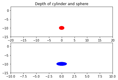
We are going to examine the magnetic anomaly, \(\Delta B_z\), caused by a sphere and a horizontal cyclinder at \(10\,m\) depth. For that, Poissons relation will be used. For this exercise, it is assumed that the magnetic field of the Earth, \(H\), as well as the magnetic fields from the objects, \(B\), are parallel. This is being done as follows:

import numpy as np
import matplotlib.pyplot as plt

# Depth of the objects
z_sphere1 = 10.0 # in [m]
z_cylinder1 = 10.0 # in [m]

# Radius of the objects
R_sphere=1.0 # in [m]
R_cylinder=1.0 # in [m]

sphere = plt.Circle((0, -z_sphere1), R_sphere, color='r')
cylinder = plt.Circle((0, -z_cylinder1), R_cylinder, color='blue')

fig, ax = plt.subplots(2)
ax[0].set_title('Depth of cylinder and sphere')
ax[0].set_xlim(-20,20)
ax[0].set_ylim(-15,2)
ax[0].add_patch(sphere)
ax[1].set_xlim(-10,10)
ax[1].set_ylim(-15,2)
ax[1].add_patch(cylinder)

<matplotlib.patches.Circle at 0x1a96875bf40>

Defining the vertical magnetic density gradient is done using Poisson’s relation. For a sphere, this is being done using the equation

\[B_{sphere} = \frac{\mu}{3} R_{sphere}^3 dM_z \frac{2 z_{sphere}^2 - x^2}{(z_{sphere}^2 + x^2)^{5/2}}\]

\[B_{cylinder} = \frac{\mu}{2}R_{cylinder}^2 dM_z \frac{ z_{cylinder}^2 - x^2}{(z_{sphere}^2 + x^2)^2}\]

# Magnetic permeability constant
mu=4.0*np.pi*10e-7

# Magnetization contrast [A/m]
dMz = 1.0e-3

# calculating B field of magnetisation
x=np.linspace(-30.0,30.0,100)
dBz1_sphere=(mu/3.0)*R_sphere**3*dMz*(2.0*z_sphere1**2-x**2)/(z_sphere1**2+x**2)**(5.0/2.0)
dBz1_cylinder=(mu/2.0)*R_cylinder**2*dMz*(z_cylinder1**2-x**2)/(z_cylinder1**2+x**2)**2

plt.xlabel(r'$x$ [m]')
plt.ylabel(r'$\Delta B_z$ [T]')
plt.title('Magnetic anomaly for objects at 10m depth')
plt.plot(x,dBz1_cylinder,'k', label = 'Anomaly by cylinder')
plt.plot(x,dBz1_sphere,'r', label = 'Anomaly by sphere')
plt.legend()
plt.grid()
plt.show()

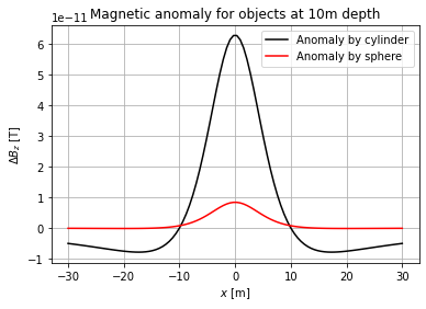
Examining the above plot with regards to \(\Delta B_z\), it can be seen that the magnetic anomaly very much depends on the shape of the object.

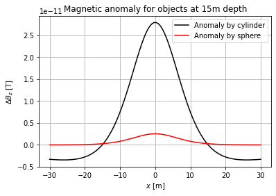
Now, we are going to examine what happens if both objects were lying deeper.

z_sphere2 = 15.0 # in [m]
z_cylinder2 = 15.0 # in [m]

x=np.linspace(-30.0,30.0,100)
dBz2_sphere=(mu/3.0)*R_sphere**3*dMz*(2.0*z_sphere2**2-x**2)/(z_sphere2**2+x**2)**(5.0/2.0)
dBz2_cylinder=(mu/2.0)*R_cylinder**2*dMz*(z_cylinder2**2-x**2)/(z_cylinder2**2+x**2)**2

plt.xlabel(r'$x$ [m]')
plt.ylabel(r'$\Delta B_z$ [T]')
plt.title('Magnetic anomaly for objects at 15m depth')
plt.plot(x,dBz2_cylinder,'k', label = 'Anomaly by cylinder')
plt.plot(x,dBz2_sphere,'r', label = 'Anomaly by sphere')
plt.legend()
plt.grid()
plt.show()

## To compare
fig, axs = plt.subplots(2, figsize = (10,5))

fig.suptitle('Vertically stacked subplots')
axs[0].plot(x,dBz1_sphere,'k', label = 'Anomaly by 10m deep sphere')
axs[0].plot(x,dBz2_sphere,'r', label = 'Anomaly by 15m deep sphere')
plt.xlabel(r'$x$ [m]')
plt.ylabel(r'$\Delta B_z$ [T]')

axs[1].plot(x,dBz1_cylinder,'k', label = 'Anomaly by 10m deep cylinder')
axs[1].plot(x,dBz2_cylinder,'r', label = 'Anomaly by 15m deep cylinder')
axs[0].legend()
axs[1].legend()

plt.xlabel(r'$x$ [m]')
plt.ylabel(r'$\Delta B_z$ [T]')
axs[0].grid()
axs[1].grid()

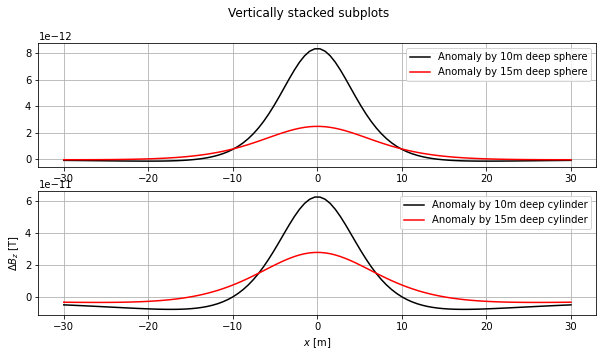
We can observe that the deeper the object, the smaller the magnetic anomaly becomes as well as more spread out.