Functions

Mathematics for Geoscientists

Basic definitions

Let us give a somewhat informal definition of a function.

Let \(\mathcal{D}\) and \(\mathcal{C}\) be non-empty sets and let \(f\) be a rule by which every element \(x \in \mathcal{D}\) is assigned a unique element \(y \in \mathcal{C}\). The ordered triple \((\mathcal{D}, \mathcal{C}, f)\) is called a function (also map or mapping). We write \(f: \mathcal{D} \to \mathcal{C}\).

Note

What that means is that the following three functions are all different despite their assignment \(f\) being the same:

\[\begin{split} \begin{aligned} f_1 : \mathbb{R} \to \mathbb{R}, \quad & f_1(x) = x^2 \\ f_2 : \mathbb{R} \to [0, \infty), \quad & f_2(x) = x^2 \\ f_3 : (- \infty, 0) \to (0, \infty), \quad & f_3(x) = x^2 \end{aligned}\end{split}\]

Functions \((\mathcal{D}_1, \mathcal{C}_1, f_1)\) and \((\mathcal{D}_2, \mathcal{C}_2, f_2)\) are equal iff \(\mathcal{D}_1 = \mathcal{D}_2, \mathcal{C}_1 = \mathcal{C}_2, f_1 = f_2\).

• \(\mathcal{D(f)}\) is called the domain of the function \(f\)

• \(\mathcal{C(f)}\) is called the codomain of the function \(f\)

• \(f(x)\) is the value (sometimes called output) of \(f\) at point \(x\)

Example:

Fig. 1 Left is a function, right is not!

The figure on the left shows a function where \( a \mapsto f(a) = 1, b \mapsto f(b) = 2, c \mapsto f(c)=2 \). The figure on the right does not represent a function since \(c\) is assigned both \(2\) and \(4\).

Cartesian (Descartes) product

The Cartesian product \(A \times B\) of two sets \(A\) and \(B\) is the set of all ordered pairs \((a, b)\) where \(a \in A, b \in B\). That is,

\[ A \times B = \{ (a, b) : a \in A, b \in B \}. \]

An example is the Cartesian plane,

\[ \mathbb{R}^2 = \mathbb{R} \times \mathbb{R} = \{ (x, y) : x, y \in \mathbb{R} \}. \]

Graph

The graph of the function is the set

\[ G(f) := \{ (x, f(x)) : x \in \mathcal{D} \}. \]

Therefore, \( G(f) \subseteq \mathcal{D} \times \mathcal{C} = \{ (d, c) : d \in \mathcal{D}, c \in \mathcal{C} \} \) .

From above examples we have the following graphs:

import matplotlib.pyplot as plt


fig, ax = plt.subplots(1, 2, figsize=(8, 3), sharey=True)

ax[0].scatter(['a', 'b', 'c'], y = [1, 2, 2])
ax[0].set_ylabel('$f(x)$')

ax[1].scatter(['a', 'b', 'c', 'c'], y = [1, 2, 2, 4], zorder=10)
ax[1].plot(['c', 'c'], [0, 4], '--k', alpha=0.3)
ax[1].set_title('Not a graph of a function!')

for i in [0, 1]:
    ax[i].set_yticks([1, 2, 3, 4])
    ax[i].spines['right'].set_visible(False)
    ax[i].spines['top'].set_visible(False)
    ax[i].set_ylim(0.8, 4.2)
    ax[i].set_xlabel('x')

plt.show()

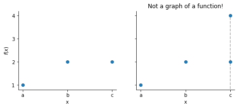
The graph on the right is not a graph of a function because two points lie on the vertical line drawn through \(c\), i.e. \(c\) is assigned two different values \(f(c)\). This is a contradiction to our definition of a function. Sometimes this is called the vertical line test.

Restriction

Let \(f : \mathcal{D} \to \mathcal{C}\) be a function and let \(A \subseteq \mathcal{D}\). We can define a restriction of \(f\) to the domain of \(A\) as \(\left.f\right|_A : A \to \mathcal{C}\) with \(\left.f\right|_A (x) = f(x), \forall x \in A\).

Image

\(\phantom{title}\)

Source: Wikipedia

Let \(f : \mathcal{D} \to \mathcal{C}\) be a function and let \(A \subseteq \mathcal{D}\). The image of a subset \(A\) under \(f\) is the set \(f(A) \subseteq \mathcal{C}\) such that:

\[ f(A) := \{ f(x) : x \in A \} \subseteq \mathcal{C}. \]

If \(A = \mathcal{D}\), i.e. the entire domain, we call the set \(f(D)\) the image or range of \(f\). In other words, the image is a set of all values that \(f(x)\) can take for all \(x\) in the domain.

From our example of a function above (left figure), let us take \(A = \{ a, c \}\). The image of a subset \(A\) is then:

\[ f(A) = \{ f(x) : x \in A \} = \{ \underbrace{f(a)}_{=1}, \underbrace{f(b)}_{=2} \} = \{ 1, 2 \}.\]

Similarly for the entire domain:

\[ f(D) = \{ f(x) : x \in \mathcal{D} \} = \{ \underbrace{f(a)}_{=1}, \underbrace{f(b)}_{=2}, \underbrace{f(c)}_{=2} \} = \{ 1, 2 \}. \]

Inverse image

Let \(f : \mathcal{D} \to \mathcal{C}\) be a function and let \(E \subseteq \mathcal{C}\). The inverse image (or preimage) of \(E\) under function \(f\) is the set

\[ f^{-1}(E) := \{ x \in \mathcal{D} : f(x) \in E \} \subseteq \mathcal{D}. \]

If we take \(E = \mathcal{C}\), then \(f^{-1}(\mathcal{C}) = \mathcal{D}\). In other words, we are looking for the values \(x \in \mathcal{D}\) for which \(f(x)\) takes specified values.

Again from the example above, let us consider \( E_1 = \{ 1 \}, E_2 = \{ 2 \}, E_3 = \{ 1, 2 \} \):

\[\begin{split} f^{-1}(E_1) = \{ x \in \mathcal{D} : f(x) \in E_1 \} = \{ x \in \mathcal{D} : f(x) = 1 \} = \{ a \} \\ f^{-1}(E_2) = \{ x \in \mathcal{D} : f(x) \in E_2 \} = \{ x \in \mathcal{D} : f(x) = 2 \} = \{ b, c \} \end{split}\]

Or some may appreciate a more applied example: let \(f: \mathbb{R} \to \mathbb{R}\) be a function with \(f(x) = x^2\), then

\[\begin{split} f([0, \infty)) = [0, \infty), \qquad f( (- \infty, 0] ) = [0, \infty) \\ f^{-1}([0, \infty)) = \mathbb{R}, \qquad f^{-1}((- \infty, 0)) = \emptyset. \end{split}\]

The last point means that there are no \(x \in \mathbb{R}\) such that \(f(x) = x^2\) is a negative number.

\(\phantom{title}\)

Or a more applied example: consider \(f: \mathbb{R} \to \mathbb{R}\) where \(f(x) = x - 5\) (we can simply write \(x \mapsto x - 5\)) and \(A = (-3, 1]\). Let us find the preimage \(f^{-1}(A)\) graphically and by calculating it.

\[\begin{split} \begin{aligned} f^{-1}(A) & = \{ x \in \mathbb{R} : f(x) \in A \} \\ & = \{ x \in \mathbb{R} : x - 5 \in (-3, 1] \} \\ & = \{ x \in \mathbb{R} : -3 < x - 5 \leq -1 \} \end{aligned} \end{split}\]

\[\begin{split} \begin{aligned} x - 5 > -3 \quad & \text{and} \quad x - 5 \leq -1 \\ x > 2 \quad & \text{and} \quad x \leq 4 \end{aligned}\end{split}\]

\[\begin{split} \begin{aligned} & \implies x \in (2, 4] \\ & \implies f^{-1}(A) = (2, 4] \end{aligned}\end{split}\]

This agrees with our findings on the graph.

Real functions

If \(\mathcal{D}\) and \(\mathcal{C}\) are subsets of \(\mathbb{R}\) then we call a function \(f : \mathcal{D} \to \mathcal{C}\) a real-valued function of a real variable or, simply, a real function.

The largest subset of \(\mathbb{R}\) for which the function \(f\) is defined is called the natural domain.

Examples. We give further examples in the notebook elementary_functions.

Function	Natural domain	Image
\( f(x) = x^2 \)	\( \mathbb{R} \)	\( [0, + \infty) \)
\( f(x)=\sqrt{x} \)	\( [0, + \infty) \)	\( [0, + \infty) \)
\( f(x) = \frac{1}{x} \)	\( \mathbb{R} \backslash \{ 0 \} \)	\( (- \infty, 0) \cup (0, + \infty) \)

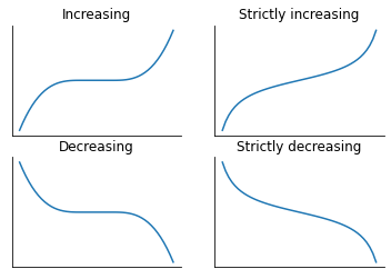
Monotonic functions

Many useful properties of real functions can easily be seen on the graph of the function. One of those is whether a function is monotonic, i.e. whether it is always increasing or decreasing on the whole domain. For a function \(f : A \to \mathbb{R}, A \subseteq \mathbb{R}\), we say that it is:

• increasing on \(A\) if \( (x_1 < x_2) \Rightarrow (f(x_1) \leq f(x_2)) \) for all \( x_1, x_2 \in A \)

• strictly increasing on \(A\) if \( (x_1 < x_2) \Rightarrow (f(x_1) < f(x_2)) \) for all \( x_1, x_2 \in A \)

• decreasing on \(A\) if \( (x_1 < x_2) \Rightarrow (f(x_1) \geq f(x_2)) \) for all \( x_1, x_2 \in A \)

• strictly decreasing on \(A\) if \( (x_1 < x_2) \Rightarrow (f(x_1) > f(x_2)) \) for all \( x_1, x_2 \in A \)

import numpy as np


def f(x):
    if x <= 0:
        y = x**3 + 1
    elif x <= 1:
        y = 1
    else:
        y = (x-1)**3 + 1
    
    return y


titles = [['Increasing', 'Strictly increasing'], 
          ['Decreasing', 'Strictly decreasing']]
    
x1 = np.linspace(-2, 3, 50)
x2 = np.linspace(-1.3, 1.3, 50)

fig, ax = plt.subplots(2, 2)

ax[0, 0].plot(x1, list(map(f, x1)))
ax[0, 1].plot(x2, np.tan(x2))
ax[1, 0].plot(x1, -np.array(list(map(f, x1))))
ax[1, 1].plot(x2, -np.tan(x2))

for i in range(2):
    for j in range(2):
        ax[i, j].spines['right'].set_visible(False)
        ax[i, j].spines['top'].set_visible(False)
        ax[i, j].set_title(titles[i][j])
        ax[i, j].set_xticks([])
        ax[i, j].set_yticks([])

plt.show()

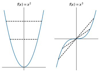
Even and odd functions

Even and odd functions satisfy particular symmetry relations. A function \(f : A \to \mathbb{R}, A \subseteq \mathbb{R}\) is:

• even on \(A\) if \(f(-x) = f(x)\) for all \(x \in A\)

• odd on \(A\) if \(f(-x) = -f(x)\) for all \(x \in A\)

The names ‘even’ and ‘odd’ originate from the power function \(f(x) = x^n\), which is even for even \(n\) and odd for odd \(n\). For example, \(f(x)=x^2\) and \(f(x)=x^3\) below:

x = np.linspace(-2, 2, 100)
y1 = x**2
y2 = x**3 / 2

fig, ax = plt.subplots(1, 2)

ax[0].plot(x, y1)
ax[1].plot(x, y2)

ax[0].plot([-1.4, 1.4], [1.4**2, 1.4**2], '--k')
ax[0].plot([-1.8, 1.8], [1.8**2, 1.8**2], '--k')
ax[1].plot([-1.4, 1.4], [-1.4**3 / 2, 1.4**3 /2], '--k')
ax[1].plot([-1.8, 1.8], [-1.8**3 / 2, 1.8**3 /2], '--k')

ax[0].set_title(r'$f(x) = x^2$')
ax[1].set_title(r'$f(x) = x^3$')

for i in range(2):
    ax[i].spines['left'].set_position('zero')
    ax[i].spines['bottom'].set_position('zero')
    ax[i].spines['right'].set_visible(False)
    ax[i].spines['top'].set_visible(False)
    ax[i].set_yticks([])
    ax[i].set_xticks([])

plt.show()