Common Mid-point Gather
Contents
Common Mid-point Gather#
Practical Seismic Data Processing Geophysical Analysis Group Project
What is it?#
Common mid-point (CMP) gather is a collection of traces that share a common mid-point (often also referred to as CDP, common depth-point, when the layer is horizontal).
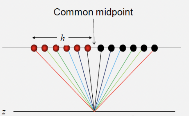
Different shots have information on the same midpoints. Reordering (sorting) them can produce data with the same midpoints, which provide redundant information on reflection points. The redundancy is exploited in velocity analysis and stacking.
Traces are sorted by surface geometry to approximate a single reflection point in the earth.
Data from several shots and receivers are combined into a single gather.
The traces are sorted by offset in order to perform velocity analysis for data processing and hyperbolic moveout correction.
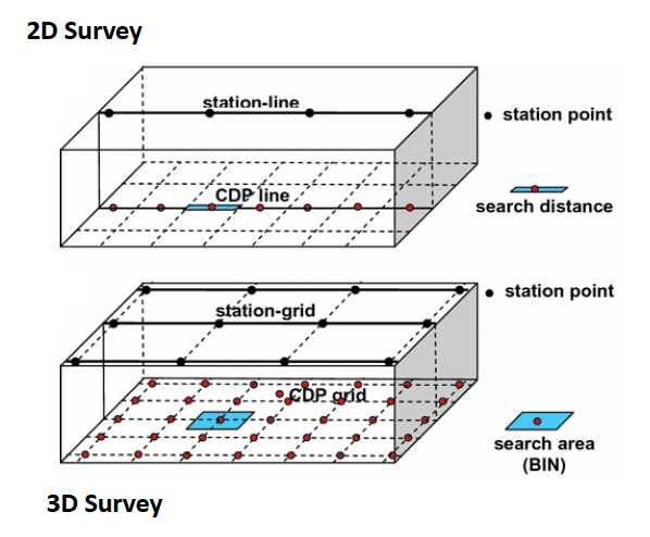
Survey Geometries#
Survey area is divided into equally sized CMP bins. This process is often referred to “binning”. Traces whose mid-point falls within that bin are assigned to that CMP (with the total number of traces per bin being our survey fold!). This is straightforward for marine surveys with simple geometries, where the CMP bins are usually spaced at half the receiver (group) interval.
where \(\text{NF}\) is no. of fold; \(\text{NC}\) is the number of channel; \(X_{R}\) is the receiver interval; \(X_{S}\) is the source interval.
For 3D surveys this will take the form of a regular grid.
Practice 1#
A marine seismic survey is carried out using a shot interval of \(20\,m\), and a cable containing \(120\) non-overlapping hydrophone groups with a spacing of \(10\,m\). The hydrophones in water are at a depth of \(8\,m\).
What is the maximum fold of the survey?
What is the midpoint spacing?
NC = 120
X_r = 10
X_s = 20

def max_fold(NC, X_r, X_s):
    NF = X_r / (2 * X_s) * NC
    return NF

print("The maximum fold of the survey is", int(max_fold(NC, X_r, X_s)),".")
The maximum fold of the survey is 30 .
X_r = 10

def midpt_spacing(X_r):
    return X_r/2

print("The midpoint spacing is", int(midpt_spacing(X_r)),"m.")
The midpoint spacing is 5 m.
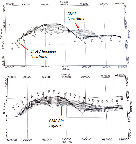
Complex Survey Geometries#
For less simple survey geometries, binning can become a lot more difficult. More complex bin arrangements have to be designed. This may result in irregularly shaped bins, whilst trying to maintain even fold, trace-offset distribution and trace-azimuth distribution throughout the survey area. Complex survey geometries are the most common in land surveying.
Reference#
2022 notes and practical from Lecture 2 of the module ESE 60023 Seismic Processing and Lecture 4 of the module ESE 70015 Advance Seismic Processing.