Elementary functions 2

Mathematics for Geoscientists

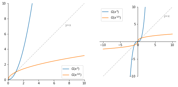
Now that we know what an inverse function is, let us think about the inverse functions of elementary functions we explored in a previous notebook.

Roots

import numpy as np
import matplotlib.pyplot as plt


x1 = np.linspace(0, 10, 101)
x2 = np.linspace(-10, 10, 101)

fig, ax = plt.subplots(1, 2, figsize=(10, 5))

ax[0].plot(x1, x1**2, label=r'$G(x^2)$')
ax[0].plot(x1, np.sqrt(x1), label=r'$G(x^{1/2})$')
ax[0].set_xlim(0, 10)
ax[0].set_ylim(0, 10)

ax[1].plot(x2, x2**3, label=r'$G(x^3)$')
ax[1].plot(x2, np.cbrt(x2), label=r'$G(x^{1/3})$')
ax[1].set_ylim(-10, 10)
ax[1].set_yticks([-10, -5, 5, 10])

for i in range(2):
    ax[i].plot(x2, x2, '--k', alpha=0.2)
    ax[i].text(7.5, 7, 'y=x', alpha=0.5)
    ax[i].set_aspect('equal')
    ax[i].spines['left'].set_position('zero')
    ax[i].spines['bottom'].set_position('zero')
    ax[i].spines['right'].set_visible(False)
    ax[i].spines['top'].set_visible(False)
    ax[i].legend(loc='best')
    
plt.show()

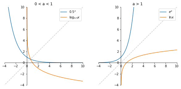
Logarithmic functions

The exponential function \(f: \mathbb{R} \to (0, + \infty), f(x)=a^x\) is an injection because it is strictly increasing and it is a surjection because its image is \(f(\mathbb{R}) = (0, + \infty)\). Therefore, it is a bijection and the inverse function \(f^{-1} : (0, + \infty) \to \mathbb{R}\) exists.

We denote this inverse function as \(\log_a x := f^{-1}(x)\) and we call it the logarithm with base a.

We call a logarithm with base \(e\) the natural logarithm and define it as:

\[ \ln x := \log_e x \]

Properties

Domain: \((0, + \infty)\), range: \(\mathbb{R}\)

\[ \log_a x = y \implies x = a^y \]

\[ (f \circ f^{-1})(y) = a^{\log_a y} = y, \forall y > 0 \]

\[ (f^{-1} \circ f)(x) = \log_a a^x = x, \forall x \in \mathbb{R} \]

For all \(x, y \in (0, + \infty), a, b, c \in (0, 1) \cup (1, + \infty)\):

\[ \log_a 1 = 0 \]

Since the exponential function maps a sum to a product, i.e. \(a^{x+y} = a^x a^y\), the logarithmic function maps a product to a sum:

\[\begin{split} \begin{align} \log_a (xy) & = \log_a x + \log_a y \\ \log_a \frac{x}{y} & = \log_a x - \log_a y \end{align}\end{split}\]

\[\begin{split} \begin{align} \log_a x^\alpha & = \alpha \log_a x \\ \log_{a^\beta} x & = \frac{1}{\beta} \log_a x \end{align} \end{split}\]

Change of base:

\[ \log_b c = \frac{\log_a c}{\log_a b} \]

x1 = np.linspace(-10, 10, 201)
x2 = np.linspace(0.001, 10, 301)

fig, ax = plt.subplots(1, 2, figsize=(10, 5))

ax[0].plot(x1, 0.5**x1, label=r'$0.5^x$')
ax[0].plot(x2, np.log(x2)/np.log(0.5), label=r'$\log_{0.5}x$')
ax[0].set_title('0 < a < 1')

ax[1].plot(x1, np.exp(x1), label=r'$e^x$')
ax[1].plot(x2, np.log(x2), label=r'$\ln x$')
ax[1].set_title('a > 1')

for i in range(2):
    ax[i].plot(x1, x1, '--k', alpha=0.2)
    ax[i].set_aspect('equal')
    ax[i].spines['left'].set_position('zero')
    ax[i].spines['bottom'].set_position('zero')
    ax[i].spines['right'].set_visible(False)
    ax[i].spines['top'].set_visible(False)
    ax[i].legend(loc='upper right')
    ax[i].set_ylim(-4, 10)
    ax[i].set_xlim(-4, 10)

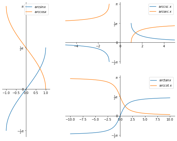
Inverse trigonometric functions

Inverse trigonometric functions are also called arcus functions so we denote them with the prefix \(\text{arc-}\), e.g. \(\arcsin x\). They are also often denoted as \(\sin^{-1} x\).

Periodic functions are not injections so they do not have inverses. Therefore, we need to restrict them to parts of their natural domain where they are strictly monotonic - here they are injections.

Then trigonometric functions with the following domain restrictions are bijections:

\[\begin{split} \begin{aligned} & \left. \sin \right|_{[-\frac{\pi}{2}, \frac{\pi}{2}]} : [-\frac{\pi}{2}, \frac{\pi}{2}] \to [-1, 1] \\ & \left. \cos \right|_{[0, \pi]} : [0, \pi] \to [-1, 1] \\ & \left. \tan \right|_{(-\frac{\pi}{2}, \frac{\pi}{2})} : (-\frac{\pi}{2}, \frac{\pi}{2}) \to \mathbb{R} \\ & \left. \csc \right|_{(-\frac{\pi}{2}, 0) \cup (0, \frac{\pi}{2})} : (-\frac{\pi}{2}, 0) \cup (0, \frac{\pi}{2}) \to (- \infty, -1) \cup (-1, + \infty) \\ & \left. \sec \right|_{(0, \frac{\pi}{2}) \cup (\frac{\pi}{2}, \pi)} : (0, \frac{\pi}{2}) \cup (\frac{\pi}{2}, \pi) \to (- \infty, -1) \cup (-1, + \infty) \\ & \left. \cot \right|_{(0, \pi)} : (0, \pi) \to \mathbb{R} \end{aligned}\end{split}\]

so we can define their inverse functions:

\[\begin{split} \begin{aligned} & \arcsin : [-1, 1] \to [-\frac{\pi}{2}, \frac{\pi}{2}] \\ & \arccos : [-1, 1] \to [0, \pi] \\ & \arctan : \mathbb{R} \to (-\frac{\pi}{2}, \frac{\pi}{2}) \\ & \text{arccsc} : (- \infty, -1) \cup (-1, + \infty) \to (-\frac{\pi}{2}, 0) \cup (0, \frac{\pi}{2}) \\ & \text{arcsec} : (- \infty, -1) \cup (-1, + \infty) \to (0, \frac{\pi}{2}) \cup (\frac{\pi}{2}, \pi) \\ & \text{arccot} : \mathbb{R} \to (0, \pi) \end{aligned}\end{split}\]

# for demonstration purposes will suppress warnings when plotting
import warnings; warnings.simplefilter('ignore')

ax = [0, 0, 0]

fig = plt.figure(constrained_layout=True, figsize=(10, 8))
gs = plt.GridSpec(2, 2, width_ratios=[1.3, 3], height_ratios=[1, 1])

ax[0] = fig.add_subplot(gs[:, 0])
ax[1] = fig.add_subplot(gs[0, 1])
ax[2] = fig.add_subplot(gs[1, 1])

x = np.linspace(-1, 1, 101)
ax[0].plot(x, np.arcsin(x), label=r'$\arcsin x$')
ax[0].plot(x, np.arccos(x), label=r'$\arccos x$')

# will include 0 to separate lines joining
x = np.concatenate((np.linspace(-5, -1, 100), [0], np.linspace(1, 5, 100)))
ax[1].plot(x, np.arcsin(1/x), label=r'arccsc $x$')
ax[1].plot(x, np.arccos(1/x), label=r'arcsec $x$')

x = np.linspace(-10, 10, 201)
ax[2].plot(x, np.arctan(x), label=r'$\arctan x$')
ax[2].plot(x, np.pi/2 - np.arctan(x), label=r'arccot $x$')

for i in range(3):
    ax[i].spines['left'].set_position('zero')
    ax[i].spines['bottom'].set_position('zero')
    ax[i].spines['right'].set_visible(False)
    ax[i].spines['top'].set_visible(False)
    ax[i].legend(loc='best')
    ax[i].set_yticks(np.pi * np.array([-2, -1.5, -1, -0.5, 0, 0.5, 1, 1.5, 2]))
    ax[i].set_yticklabels(['$-2\pi $', r'$-\frac{3}{2} \pi $', r'$-\pi$', 
                    r'$-\frac{1}{2}\pi$', '0', r'$\frac{1}{2}\pi$', 
                    r'$\pi$', r'$\frac{3}{2}\pi$', r'$2\pi$'])
    
ax[0].set_xlim(-1.2, 1.2)
ax[0].set_ylim(-1.8, 3.3)

ax[1].set_xlim(-5, 5)
ax[1].set_ylim(-1.7, 3.3)

ax[2].set_ylim(-1.7, 3.3)

plt.show()

Properties

For a more complete list of properties and their visualisation, visit Wikipedia. Here we will name a few.

Complementary angles:

\[ \arccos x = \frac{\pi}{2} - \arcsin x, \quad \text{arccot} x = \frac{\pi}{2} - \arctan x, \quad \text{arccsc} x = \frac{\pi}{2} - \text{arcsec} x \]

Reciprocal arguments:

\[\begin{split} \begin{aligned} \arccos \left( \frac{1}{x} \right) = \text{arcsec} x, \quad & \quad \text{arcsec} \left( \frac{1}{x} \right) = \arccos x \\ \arcsin \left( \frac{1}{x} \right) = \text{arccsc} x, \quad & \quad \text{arccsc} \left( \frac{1}{x} \right) = \arcsin x \\ \text{if } x > 0: \arctan \left( \frac{1}{x} \right) = \text{arccot} x, \quad & \quad \text{arccot} \left( \frac{1}{x} \right) = \arctan x \\ \text{if } x < 0: \arctan \left( \frac{1}{x} \right) = \text{arccot} x - \pi, \quad & \quad \text{arccot} \left( \frac{1}{x} \right) = \arctan x + \pi \\ \end{aligned} \end{split}\]

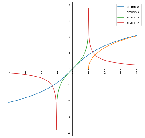
Inverse hyperbolic functions

Inverse hyperbolic functions are also called area functions so we denote them with the prefix \(\text{ar-}\), e.g. \(\text{arsinh} x\). They are also often denoted as \(\sinh^{-1} x\), for example.

Hyperbolic functions

\[\begin{split} \begin{align} \sinh : \mathbb{R} \to \mathbb{R} \\ \left. \cosh \right|_{[0, + \infty)} : [0, + \infty) \to [1, + \infty) \\ \tanh : \mathbb{R} \to (-1, 1) \\ \coth : \mathbb{R} \backslash \{ 0 \} \to (- \infty, -1) \cup (1, + \infty) \end{align} \end{split}\]

are bijections, so we can define their inverses:

\[\begin{split} \begin{align} \text{arsinh} := \sinh ^{-1} : \mathbb{R} \to \mathbb{R} \\ \text{arcosh} := \left ( \left. \cosh \right|_{[0, + \infty)} \right)^{-1} : [1, + \infty) \to [0, + \infty) \\ \text{artanh} := \tanh^{-1} : (-1, 1) \to \mathbb{R} \\ \text{arcoth} := \coth^{-1} : (- \infty, -1) \cup (1, + \infty) \to \mathbb{R} \backslash \{ 0 \} \end{align} \end{split}\]

where

\[\begin{split} \text{arsinh} x = \ln ( x + \sqrt{x^2 + 1} ), \qquad \text{arcosh} x = \ln (x + \sqrt{x^2 - 1}), \\ \text{artanh} x = \frac{1}{2} \ln \left( \frac{1+x}{1-x} \right ), \qquad \text{arcoth} x = \frac{1}{2} \ln \left( \frac{x+1}{x-1} \right ) \end{split}\]

Derivation of arcosh \(x\)

For demonstration purposes let us derive the above equation for \(\text{arcosh} x\). Recall that \(\cosh x = \frac{e^x + e^{-x}}{2}\). Let that equal some \(y\), so that \(\frac{e^x + e^{-x}}{2} = y\) or \(e^x + e^{-x} - 2y = 0\). Now let \(u = e^x\) and multiply both sides by \(u\). We get:

\[ u^2 - 2uy + 1 = 0., \]

which is a simple quadratic equation with solutions:

\[ u_{1,2} = y \pm \sqrt{y^2 - 1}. \]

But since \(u = e^x > 0\) the only possible solution is

\[ u = e^x = y + \sqrt{y^2 - 1}. \]

We take the natural logarithm of both sides:

\[ x = \ln \left ( y + \sqrt{y^2 -1} \right ) \]

fig = plt.figure(figsize=(10, 8))
ax = plt.gca()

x = np.linspace(-4, 4, 201)
plt.plot(x, np.log(x + np.sqrt(x**2 + 1)), label=r'arsinh $x$')

x = np.linspace(1, 4, 101)
plt.plot(x, np.log(x + np.sqrt(x**2 - 1)), label=r'arcosh $x$')

x = np.linspace(-0.999, 0.999, 200)
plt.plot(x, np.log((1+x)/(1-x)) / 2, label=r'artanh $x$')

# will include 0 to avoid joining lines, this returns an error
x = np.concatenate((np.linspace(-4, -1.001, 100), [0], np.linspace(1.001, 4, 100)))
plt.plot(x, np.log((x+1)/(x-1)) / 2, label=r'artanh $x$')

ax.spines['left'].set_position('zero')
ax.spines['bottom'].set_position('zero')
ax.spines['right'].set_visible(False)
ax.spines['top'].set_visible(False)
ax.set_aspect('equal')
ax.legend(loc='best')

plt.show()