Work and Energy#

Mechanics Physical Processes

import numpy as np
%matplotlib inline
import matplotlib.pyplot as plt
from matplotlib import animation, rc
from IPython.display import HTML

Work-energy theorem#

Mathematically, work-energy theorem is stated as the following:

W_{12} = \int_{x_{1}}^{x_{2}} F (x) d x

where $W_{12}$ is the work done on a body by the force $F$ as the body moves from point $x_{1}$ to $x_{2}$ .

$W_{12}$ is equal to the change in energy when the body moves from $x_{1}$ to $x_{2}$ .

Forms of energy#

Kinetic energy#

K E = \frac{1}{2} m v^{2}

where $m$ is mass, $v$ is velocity

Potential energy#

Gravitational potential energy#

G P E (x) = m g x

where $m$ is mass, $g$ is gravitational acceleration, $x$ is the height above a reference point where $x = 0$

Elastic potential energy#

E P E (x) = \frac{1}{2} k x^{2}

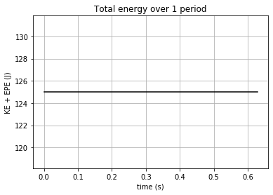
Note: total energy is constant over time

Equipartition of Energy#

The principle of equipartition of energy states that at thermal equilibrium, magnitude of different forms of energy are equal on average.

Tutorial Problem 3.6#

Consider a body connected to a spring, oscillating according to $x (t) = x_{0} \cos (\sqrt{\frac{k}{m}} t)$ .

Derive expressions for the elastic potential energy of the body as a function of time, for the kinetic energy of the body as a function of time, and for the total energy of the body as a function of time.

Draw a simple sketch of these energies as a function of time. What is the average value of $K E$ , and the average value of $E P E$ , over one period? You should find that the average values of $K E$ and $E P E$ are equal.

g = 9.81 # m/s2

# input arbitrary numbers
m = 10 # mass kg
k = 1e3 # spring constant N/m
x0 = 0.5 # m

T = 2 * np.pi * np.sqrt(m/k) # period in simple harmonic motion

print("Period = %.2f" % T)

t = np.linspace(0, T, 500)

X = x0 * np.cos(np.sqrt(k/m)*t)

dxdt = -x0 * np.sqrt(k/m) * np.sin(np.sqrt(k/m)*t)

epe = 0.5 * k * X**2

ke = 0.5 * m * dxdt**2

average_epe = np.sum(epe)/len(epe)

average_ke = np.sum(ke)/len(ke)

print("Average EPE = %.dJ" % (average_epe))
print("Average KE = %.dJ" % (average_ke))

# plot figures of EPE, KE, and total energy over 1 period

fig = plt.figure(figsize=(6,4))

plt.plot(t, ke+epe, 'k')
plt.xlabel('time (s)')
plt.ylabel('KE + EPE (J)')
plt.title('Total energy over 1 period')
plt.grid(True)

plt.show()

Period = 0.63
Average EPE = 62J
Average KE = 62J

nframes = len(t)

# Plot background axes
fig, axes = plt.subplots(1,3, figsize=(15, 10))

line1, = axes[0].plot([], [], 'ko', lw=2)
line2, = axes[1].plot([], [], 'ro', lw=2)
line3, = axes[2].plot([], [], 'bo', lw=2)


axes[0].set_xlim(-0.1, 0.1)
axes[0].set_ylim(-0.6, 0.6)
axes[0].set_ylabel('displacement (m)')
axes[0].set_title('Motion of body over 1 period')
axes[1].set_xlim(-0.1, 0.1)
axes[1].set_ylim(0, 130)
axes[1].set_ylabel('EPE (J)')
axes[1].set_title('Elastic potential energy over 1 period')
axes[2].set_xlim(-0.1, 0.1)
axes[2].set_ylim(0, 130)
axes[2].set_ylabel('KE (J)')
axes[2].set_title('Kinetic energy over 1 period')
    
lines = [line1, line2, line3]

# Plot background for each frame
def init():
    for line in lines:
        line.set_data([], [])
    return lines

# Set what data to plot in each frame
def animate(i):
    
    x1 = 0
    y1 = X[i]
    lines[0].set_data(x1, y1)
    
    x2 = 0
    y2 = epe[i]
    lines[1].set_data(x2, y2)
    
    x3 = 0
    y3 = ke[i]
    lines[2].set_data(x3, y3)
    
    return lines

# Call the animator
anim = animation.FuncAnimation(fig, animate, init_func=init,
                               frames=nframes, interval=10, blit=True)

HTML(anim.to_html5_video())

References#

Course notes from Lecture 3 of the module ESE 95011 Mechanics

ESE Jupyter Material

Work and Energy

Contents