BTCS scheme
Contents
BTCS scheme#
In the FTCS scheme, we have used a forward difference at time \(t_n\) and a second order central difference for the space derivative at position \(x_j\) to obtain a recurrence equation. Instead of \(i\) shown before in the FTCS method, we have used \(j\) to denote the position.
Finite differencing requires some information before we attempt to solve it. Typically, you have
the differential equation you are applying the scheme to
the boundary conditions for the differential equation
the initial conditions of the differential equation or the condition for the differential equation at some other point in time
In this notebook, we will learn about Backward Time Centred Space method to solve ordinary differential equations.
Theory#
Heat equation#
For example, take our heat equation, that is often written more compactly as
we use the letter \( U \) to denote the temperature, letter \( t \) to denote the time and \(\alpha \) to denote the thermal diffusivity of the medium.
In three dimensions, an arbitrary function \(f\) the Laplacian operator is defined as being
Thus the dot product, i.e. \( \nabla \cdot \nabla \), similar to how we do the dot product between vectors in 3 dimensions, can be written as
We understand that to get to \( \Delta f \), we need to bring \(\nabla \cdot \nabla \) to \( f \), and thus we apply each term of \(\nabla \cdot \nabla \) to \( f \), and thus we obtain
We could easily increase or decrease the number of dimensions involved as needed for the Laplacian operator. Below we will see a two dimensional example, and then we will use a one dimensional example to illustrate the BTCS scheme.
For the normalized heat equation in two dimension, the differential equation that we have, is:
Although we have gotten rid of \( z \), then \( y \), resulting in the 1D heat equation having the position denoted through \( x \), you could replace \( x,y\) or \( z \) here with any letter. Similarly, you could use any other letter than \( U\) to denote the temperature, as long as you know that the letter represents temperature. The same goes for \( t \).
The explaination for the heat equation presented is straightforward. We know from basic classical thermodynamics that heat is transferred from locations of high temperature, i.e. higher average kinetic velocity of particles, to locations of lower temperature, i.e. lower average kinetic velocity of particles. We also know that how quickly heat is transferred depends on the temperature difference, so higher temperature difference results in faster heat transfer from one object to another, and lower temperature difference results in slower heat transfer from one object to another.
A typical example would be using a knife to slice butter. A hot knife slices easily through butter because there is a large temperature difference between the hot knife and the butter, which causes the butter to melt around the hot knife and become easier to slice. A cold knife cannot slice easily through butter because there is only small or no temperature difference between the hot knife and butter, and the heat transfer from the knife to the butter (assuming that the knife is hotter than the butter) is very slow, which causes the butter to not melt, or at least melt slowly and makes it much harder to slice.
We understand that the temperature change with time of an object affected by heat transfer from or to its surroundings is proportional to temperature difference with its surroundings. The temperature change with time of an object can be written as \( \partial U/\partial t \). The temperature difference with its surroundings can be expressed as the derivative of the temperature with respect to distance. We find that in practice, temperature change with time is actually proprotional to the second derivative of the temperature with respect to the distance, i.e. \( \partial ^2U/\partial x^2 \). Since we have proportionality, we also must have a constant of proportionality, and the constant of proportionality for our heat equation is \(\alpha \) where the \(\alpha \) here denotes the thermal diffusivity of the medium. For the generalized form, we express through the Laplacian and adapt it to our problem depending on the number of dimensions of the problem.
General:
For the normalized heat equation in three dimensions, the differential equation that we have, is:
For the normalized heat equation in two dimensions, the differential equation that we have, is:
For the normalized heat equation in one dimension, the differential equation that we have, is:
Scheme#
An important picture that summarizes the BTCS schem can be seen in the figure below:

Source: Wikipedia
Our objective is to find the point at the location \(j\) and timestep \(n+1\). The BTCS scheme means backwards in time centered in space scheme. Looking at the illustration above, we see that there are three other points linked to the point at the location \(j\) and timestep \(n+1\). As expected, we are going to use those three points, and their relative relation to the point at location \(j\) and timestep \(n+1\) that we are trying to find for our BTCS scheme.
Two of the points we are going to use are the point to the left at the location \(j-1\) and timestep \(n+1\) and the point to the right at the location \(j+1\) and timestep \(n+1\), i.e. centered in space parts of BTCS. Another point we are going to use is the point before in time at the location \(j\) and timestep \(n\). Notice that the shape of the illustration is T - shaped, with the T pointintg backwards in time, hence the name of the scheme.
Since we see that there is only a single position argument, i.e. there is only \(j\), we understand that the illustration above is for a 1D problem. We will demonstrate BTCS using a 1D problem first. You could easily adapt the equations below for 2D, 3D and even higher dimension problems.
Let’s take our classical heat transfer equation and let’s do 1D heat transfer Here we are going to use \(u\) instead of \(U\) because we are working with individual points in the matrix, which is usually represented by small letters, instead of the entire matrix, which is usually represented by a big letter.
Thus, we will have to try to solve:
To solve this, we will need to use numerical methods to find \(\partial u/\partial t\) and \(\partial ^2 u / \partial x^2 \), which can be found, using the 3 aforementioned points in the illustration. For demonstrating BTCS, let’s say that \(\alpha\) is a constant. The time derivative is going to be the same as the FTCS scheme, but unlike the FTCS scheme, the space derivative will use the points forward in time, i.e. the points at timestep \(n+1\).
Thus, we begin the BTCS scheme by writing out the relevant equations, just like with the FTCS scheme.
Applying the above to our heat equation, we can write
The above equation can be rearranged easily to make the point that we wish to obtain into the subject of the equation, i.e. \( u_{j}^{n+1} \)
We have seen how we could get our desired point \(u_{j}^{n+1}\) beginning from the heat equation. However, there are many different differential equations in nature. Supposedly we have an equation that is not too different from our heat equation here, how should we proceed to try to use to the BTCS scheme on it?
We know that for our 1D PDEs, with one spatial dimension and one time dimension, and using the Forward Euler for our time, and the Central Difference for our location, our PDE will always consists of a combination of of the terms illustrated above, and therefore can be always rearranged into the following form, no matter if we used the heat equation or not. Note that our conclusion that the PDE can be arranged into the following depends on
1D PDE with 1 spatial dimension and 1 time dimension
forward Euler method for the time derivative
central difference method for the location derivative
In terms of accuracy, because we are using the forward Euler method in time, BTCS is 1st order accurate. Because we are using the central difference method in space, BTCS is 2nd order accurate in space.
We could easily see why more terms will be required if the problem we are solving is 2 dimensional or of higher dimension, and we could see why the terms included will not be the same if we you different methods for the time or the location derivative.
Boundary conditions#
We have concluded from before that to obtain the our desired point \(u_{j}^{n+1}\), for 1 spatial dimension and 1 time dimension, using forward Euler for the time derivative, and central difference for the location derivative, we need to solve a general equation of the form
For the heat equation, we adapt the general form to become
We understand that if we could solve equations in the general form, it would not be a problem to solve the heat equation since \(\alpha \), is a material property and is usually given as a constant, or is rather trivial to solve for, and \(\Delta x\) and \(\Delta t\) are controlled by the user.
To obtain the our desired point \(u_{j}^{n+1}\), we need \(u_{j}^{n}, u_{j}^{n+1}, u_{j-1}^{n+1} \). Unlike the FTCS, where you could directly substitute to find your desired point, i.e that’s why FTCS is an explicit scheme, the BTCS scheme is an implicit scheme. In BTCS, we have a slight problem that we cannot substitute like in FTCS, because we don’t actually know \(u_{j+1}^{n+1}\) and \(u_{j-1}^{n+1} \) needed to solve for our desired point, because we only have information about the current timestep \(n\) and not the future timestep \(n+1\).
First, we know that our heat equation can also be rearranged into the following, where \(u_{j}^n\) is the subject of the equation. Any equation in the general form shown above can also be rearranged into the following form, with \({u}_{j}^n\) being the subject of the equation, with the dependent variable not neccesarily being \(u\). \(u\), the temperature is the dependent variable for the heat equation, but another quantity can be the dependent variable for another equation.
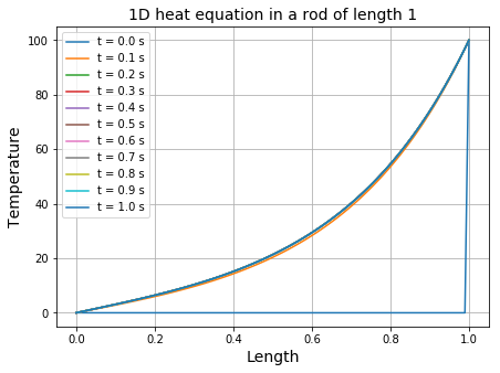
To use the boundary conditions, we need to be at the boundary. Let’s set some simple boundary conditions to illustrate our example, using the simplest Dirichlet boundary conditions for demonstration sake. Since we have a 1D problem, we are going to use a rod as an example, with temperature one end of the rod is fixed at 0 degree and the other end is fixed at 100 degrees. Let’s suppose we call the end of the rod to be \(L\). Let’s say that \(j\) increases from left to right. Our boundary conditions are:
If we adapt the above equation to our problem we can obtain that at the left end of the rod, we will ignore the term \(u_{0-1}^{n+1}\). We also note that because of our Dirichlet boundary forcing the end of the rod to be a certain temperature, the term to the right of the end i.e. \(u_{0+1}^{n+1}\), although existing, will not affect the temperature at the end of the rod.
Since we have already stated that our simple Dirichlet boundary conditions forces the temperature at the left end to be \(0\) no matter the time elapsed, we could state that
If we adapt the above equation to our problem we can obtain that at the right end of the rod, we will ignore the term \(u_{L+1}^{n+1}\).
Therefore,
For any other point in the middle, we will have:
For example, for point immediately after the left end of the rod, i.e. point where \(j=1\) we will write
and so on and so forth.
We see for the equation above that for any point that we are seeking, i.e. \( u_{j}^{n+1} \), even the points in the boundary conditions, there will be a point to the left, i.e. \(u_{j-1}^{n+1}\), and a point to the right, i.e. \(u_{j+1}^{n+1}\) and a point one timestep back, i.e. i.e. \( u_{j}^{n} \).
Let’s call the coefficient of the point we are seeking to be \( a_j \), the coefficient of the point to the left of the point we are seeking to be \( c_j \), the coefficient of the point to the right of the point we are seeking to be \( b_j \) and the coefficient for one timestep back to be \( d_j \).
For example, for \(j=5\),i.e. point where \(j=5\) we will write
Thus, we understand that for each point in the rod there will be an equation, and we could write the equations, starting from the left boundary where \(j=0\) to the the right boundary where \(j=1\) together as such, assuming that we broke the road into many discrette intervals
To apply boundary conditions, we can set the coefficient of what is out of bounds to be \(0\)
since we are using Dirichlet boundary and forcing the end of the rods to be at a specified temperature, no matter the time elapsed, as shown through, then we can set other coefficients to be \(0\) to represent that these have no effect on the temperature at the boundary.
Knowing that
We note that for
or rather
Since
Then
We can write
And instead set our \(a_0 = a_{L} 1\), at the boundary only !!!
Thus we write, keeping \(a_0 = a_{L} 1\) in mind
Thise set of equation looks like a matrix equation \(\pmb{Ax=b}\).
With \(a_0 = a_{L} 1\) in mind, we write
We also write for \(\pmb{x}\) and for \(\pmb{B}\)
Thus we write
Note that the values which were out of bounds were ignored in the construction of the matrix.
Tridiagonal matrices#
While you can solve the above through simple Gaussian elimination algorithm, Gaussian elimination may not be the best approach, at least for our 1D heat equation. We observe that for our 1D heat equation, we have something called a tridiagonal matrix.
A triagonal matrix is a type of matrix that has nonzero elements on the main diagonal, the first diagonal below this, and the first diagonal above the main diagonal only.
The better way to solve for tridiagonal matrices is actually through LU decomposition.
The result of doing LU decompostion on a tridiagonal matrix gives
Thus, to find \(\pmb{L, U}\) we need to find \(e, f\). From \(\pmb{A}\), we already know \(a, b, c\)
From the above, you should be able to observe the following relationship
For \( j = 1\), we have:
For \( j = 2, 3, 4, \ldots , L-2, L-1, L\), we have:
Implementation#
Example of BTCS applied for 1D rod with Dirichlet boundary previoulsy described:
import numpy as np
import scipy as sp
import matplotlib.pyplot as plt
import copy

## 1. Defining Parameters

L = 1             # Length of Rod
dx = 0.01         # Length of each interval of rod
n = int(L/dx - 1) # Number of Intervals = L/dx - 1
alpha = 1         # Assume alpha is 1, change based on situation, ## Suggested to be kept same as dx
dt = 0.1

## 2. Creating two matrices for representing the rod

a_before = np.zeros(shape = n)
a_after = np.zeros(shape = n)

# 3. Setting up initial conditions
a_before[0] = 0
a_before[-1] = 100 ## Python starts counting from zero

#print(a_before)

## 4. Creating our Matrix A based on what we found about a,b,c, and d

A = np.zeros(shape = (n,n))
#print(A)

for j in range(n):

    try:
            A[j][j - 1]  = -alpha/(dx ** 2)

            A[j][j] = 1/dt + 2*alpha/(dx ** 2)
            A[j][j + 1] = -alpha/(dx **2)

    except:
        continue

A[0][-1] = 0 ###### Preventing the appearanc of rogue at the upper right corner

## 5. Applying the calculate Dirichlet boundary conditions to our A

A[0,0] = 1
A[0,1] = 0
A[-1, -2] = 0
A[-1, -1] = 1
#print(A)

#print(A)

## 6. Creating L and U for LU decomposition

L = np.zeros(shape = (n,n))
U = np.zeros(shape = (n,n))

##print(L)
##print(U)

####Setting up the a1 = f1

U[0, 0] = A[0,0]
L[0, 0] = 1

#### Then setting up based on what we found about e and f from before

for j in range(1, n):

    #print("This is step ", j)

    L[j,j] = 1

    L[j,j-1] = A[j][j-1] / U[j-1][j-1]

    U[j-1,j] = A[j-1, j]

    U[j,j]   = A[j,j] - L[j, j-1] * A[j-1, j]

    ##print(L)
    ##print(U)

##7.  Completed the LU Decomposition, Proceeding from LU Decomposition to solve equation

#plt.imshow(L@U)
#plt.show()
#plt.imshow(A)
#plt.show()
#Check if L@U=A

## We note that LUx = b
## We know that for us in the heat equation will store the d0, d1, d2, etc.
## d1, d2, d3 etc. are the values from the previous timestep, so a_before
## We also know x is going to contain our values for the new timestep, without the coefficients
## We need to find x, i.e. the new timestep, using the values from the previous timestep

## We begin by using substitution to solve for L(Ux) = b, to first obtain UX
## We then proceed to use subsitution to find x from Ux

print("Temperature with initial conditions")
print(a_before)

##Starting a list to be populated by timesteps
timesteps = [a_before ]

for i in range(0, 10):

    ##Let's begin by populating our b matrix
    b = (1/dt) * copy.deepcopy(a_before)

    ##We then need to remember to apply the boundary conditions to b

    b[0]  = 0
    b[-1] = 100

    ## From Ax = b, by back subsitution, we have LUx = b
    ## We first find L(Ux) = b, we know L, and we know b, thus we can find Ux
    ## We are going to solve for Ux first, by using back substitution

    #print(b)
    #print(L)

    UX = np.zeros(n)

    for i in range(n-1, -1, -1):
        tmp = b[i]
        for j in range(n-1, i, -1):
            tmp -= UX[j]*L[i,j]

        UX[i] = tmp/L[i,i]

    #print(UX)

    ## Thus, we know that UX = [sth, sth, \ldots, sth, sth]

    ## Since the equation is U@x = UX
    ## We know U from LU factorization, and we know UX from the repvious step, thus, we can solve for x

    #print(U)
    #print(UX)

    ## We apply the same thing as before
    ## This time, we are solving for X in UX, so U@X = UX
    ## Before, we were solving for UX in LUX = b
    ## So instead of b we write UX, instead of L we write U, and instead of UX we write X

    X = np.zeros(n)

    for i in range(n-1, -1, -1):
        tmp = UX[i]
        for j in range(n-1, i, -1):
            tmp -= X[j]*U[i,j]

        X[i] = tmp/U[i,i]

    #print(X)

    ## Ok, so now we have obtained an X, which is the solution to the new timestep, let's update the timesteps.

    a_before = copy.deepcopy(X)
    a_after = np.zeros(shape = n)

    #print(a_before)
    #print(a_after)
    timesteps.append(a_before)
    ##EXTRA: I will store the A_before in a list and plot it to demonstrate the change

print("Temperature for final timestep ")
print(a_before)

#### Note: you do not neccesarily have to go through the steps outlined in the same order
#### Note: More complex simulations may require extra steps
#### Go through your derivations slowly and meticulously step by step before proceeding to code it out
#### It will save you lot's of headaches !!!
Temperature with initial conditions
[  0.   0.   0.   0.   0.   0.   0.   0.   0.   0.   0.   0.   0.   0.
   0.   0.   0.   0.   0.   0.   0.   0.   0.   0.   0.   0.   0.   0.
   0.   0.   0.   0.   0.   0.   0.   0.   0.   0.   0.   0.   0.   0.
   0.   0.   0.   0.   0.   0.   0.   0.   0.   0.   0.   0.   0.   0.
   0.   0.   0.   0.   0.   0.   0.   0.   0.   0.   0.   0.   0.   0.
   0.   0.   0.   0.   0.   0.   0.   0.   0.   0.   0.   0.   0.   0.
   0.   0.   0.   0.   0.   0.   0.   0.   0.   0.   0.   0.   0.   0.
 100.]
Temperature for final timestep
[  0.           0.31327884   0.62655768   0.93999308   1.25384584
   1.56840277   1.88396128   2.2008244    2.51929886   2.83969425
   3.16232271   3.48749887   3.81553989   4.14676567   4.48149898
   4.82006579   5.16279544   5.51002098   5.86207944   6.21931214
   6.58206501   6.95068888   7.32553985   7.70697958   8.09537568
   8.49110202   8.8945391    9.30607441   9.72610281  10.15502688
  10.59325733  11.04121339  11.49932318  11.96802415  12.4477635
  12.93899857  13.4421973   13.9578387   14.48641324  15.02842339
  15.58438405  16.15482304  16.74028162  17.34131502  17.95849291
  18.5924      19.24363654  19.91281895  20.60058035  21.30757118
  22.03445981  22.78193321  23.55069752  24.3414788   25.15502366
  25.99209999  26.8534977   27.74002941  28.65253127  29.59186375
  30.55891241  31.55458876  32.57983114  33.63560555  34.72290662
  35.84275851  36.99621589  38.18436492  39.4083243   40.66924628
  41.96831779  43.30676153  44.68583713  46.10684235  47.57111426
  49.08003054  50.63501076  52.23751772  53.88905881  55.59118745
  57.34550456  59.15366001  61.01735424  62.93833981  64.91842309
  66.95946593  69.0633874   71.23216562  73.46783962  75.77251126
  78.14834715  80.59758079  83.12251457  85.72552199  88.40904988
  91.1756207   94.0278349   96.96837338 100.        ]
plt.figure(figsize=(7,5))

for i in range(len(timesteps)):
    plt.plot(list(np.linspace(0, 1 ,n)), timesteps[i],
             label = "t = %.1f s" % (i*dt))

plt.title("1D heat equation in a rod of length 1", fontsize=14)
plt.grid(True)
plt.xlabel("Length", fontsize=14)
plt.ylabel("Temperature", fontsize=14)
plt.legend()
plt.show()
Initial guess#
The BTCS scheme is unconditionally stable, it actually does not matter what is your initial guess and the system will eventually reach stead state. However, a bad initial guess is a bad practice, and while BTCS is unconditionally stable, it is not okay to make unneccesary calculations.
Benefits of a good initial guess include
fewer steps to reach the steady state, less computational power required
less likely for the scheme to get weird erros
less likely to fall into a local minima instead of the absolute minima
For example, a good initial guess as to the final temeprature state in the rod would be that there is a steady increase in temeprature from the cold end of the rod to the hot end of the rod, with the coldest temepratures not colder than the cold end, and the hottest temeperatures not hotter than the hot end.