Ghosting

Practical Seismic Data Processing Geophysical Analysis Group Project

What is it?

In marine acquisition, the source and receiver are both towed slightly below the sea surface, this leads to a reflection from the sea surface just above the source receiver. This reflection is refered as “ghosting”.

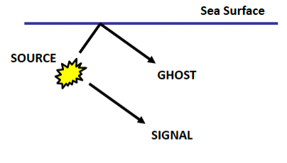
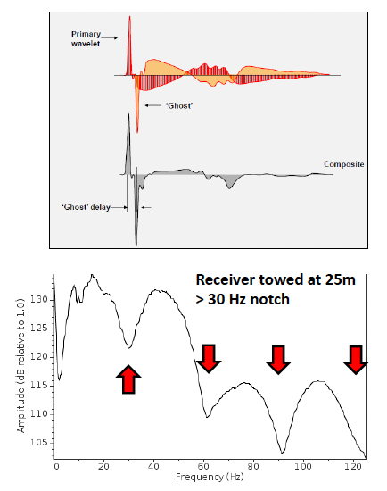
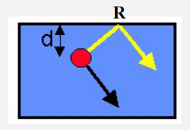
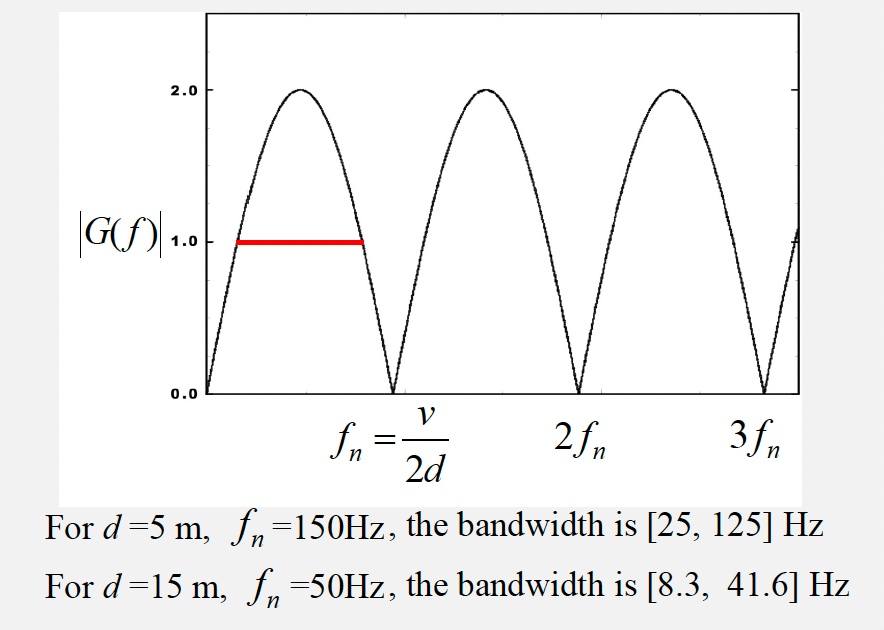
Ghosting results in a noisier trace. The interaction of these two signals also leads to regular “notches” in the frequency spectrum, which can limit the bandwidth. The location of these notches \(f_{n}\) is dependant on the depth \(d\) of the source and receivers.

\[f_{n}=\frac{v}{2d}\]

When designing survey, we need to achieve a delicate balance between the depth of the sources and receivers (deeper = quieter!) and the expected location of the notch (deeper = notch at lower frequency i.e. more reduced bandwidth!).

Specific operators can be designed to remove the ghost and balance the amplitude of the frequencies in the ghost notch during processing, Where possible may be more convenient to filter out the notched data.

Practice 1

Calculate the notch frequency when the receiver is towed at \(25\,m\).

v = 1500 #velocity of sound in water
d = 25

def notch_freq(v,d):
    return v / (2 * d)

print("The notch frequency when the receiver is towed at 25 m is", int(notch_freq(v,d)), "Hz.")

The notch frequency when the receiver is towed at 25 m is 30 Hz.

Surface Ghost in Dipole

Ghosting can be described by a two-point filter (dipole). Assumes 1D plane waves (i.e. “far field”):

\[G(z)=1+Rz^{\frac{2d}{v{\Delta}t}}\]

\[n=\frac{2d}{v{\Delta}t} \quad ; \quad z=\exp\left({-i{\omega}{\Delta}t}\right) \quad ; \quad {\omega}=2{\pi}f \]

In practice \(|R| < 1\). We refer \(n\) as time index and \(z\) as unit time delay. In the following calculation, we assume \(R = -1\).

\[G(z)=1-z^{\frac{2d}{v{\Delta}t}}\]

\[G(f)=1-\exp\left(-i\frac{4{\pi}fd}{v}\right)\]

\[G(f)=\exp\left(-i\frac{2{\pi}fd}{v}\right) \left[\exp\left(i\frac{2{\pi}fd}{v}\right) - \exp\left(-i\frac{2{\pi}fd}{v}\right)\right]\]

\[G(f)=2\sin\left(\frac{2{\pi}fd}{v}\right) \exp\left[-i\left(\frac{2{\pi}fd}{v}-\frac{{\pi}}{2}\right)\right]\]

where \(2\sin\left(\frac{2{\pi}fd}{v}\right)\) is the amplitude and \(\exp\left[-i\left(\frac{2{\pi}fd}{v}-\frac{{\pi}}{2}\right)\right]\) is the phase.

The amplitude spectrum is

\[|G(f)|=2\left|\sin\left(\frac{2{\pi}fd}{v}\right)\right|\]

Practice 2

If the Fourier Transform of the operator \(G(z)\) is

\[G(f)=2\sin\left(\frac{2{\pi}fd}{v}\right) \exp\left[-i\left(\frac{2{\pi}fd}{v}-\frac{{\pi}}{2}\right)\right]\]

Calculate the first and second notch frequency for a streamer at depth \(5\,m\) and using a velocity of water of \(1500\,m/s\).

\[\frac{2{\pi}f_{n}d}{v}=k{\pi}\quad,\quad k=0,1,2...\]

\[f_{n}=k\frac{v}{2d}\]

v = 1500
d = 5

def notch_f(k,v,d):
    return (k * v) / (2 * d)

print("The first notch frequency is", int(notch_f(1,v,d)),"Hz.")
print("The second notch frequency is", int(notch_f(2,v,d)),"Hz.")

The first notch frequency is 150 Hz.
The second notch frequency is 300 Hz.

Reference

2022 notes and practical from Lecture 3 of the module ESE 60023 Seismic Processing and Lecture 1 of the module ESE 70015 Advance Seismic Processing.