Systems of linear equations
Contents
Systems of linear equations#
Mathematics Methods 1 Geophysical Inversion Numerical Methods
Consider a general system of \(m\) linear equations with \(n\) unknowns (variables):
where \(x_i\) are unknowns, \(a_{ij}\) are the coefficients of the system and \(b_i\) are the RHS terms. These can be real or complex numbers.
Almost every problem in linear algebra will come down to solving such a system. But what does it mean to solve a system of equations?
Solution of the system#
Solving a system of equations means to find all n-tuples \((x_1, x_2, ..., x_n)\) such that substituting each one back into the system gives exactly those values given on the RHS, in the correct order. We call each such tuple a solution of the system of equations.
To solve such a system we will use basic arithmetic operations to transform our problem into a simpler one. That is, we will transform our system into another equivalent system. We say that two systems of equations are equivalent if they have the same set of solutions. In other words, the transformed system is equivalent to the original one if the transformation does not cause a solution to be lost or gained.
Three such transformations (sometimes called elementary row operations) of a system of linear equations that result in an equivalent system are:
Swapping any two equations of the system
Multiplying an equation of the system by any number different from 0
Adding an equation of the system multiplied by a scalar to another equation of the system
We will aim to use these transformations to eliminate certain unknowns from some equations. Ideally, we would like to reduce one equation to have only one unknown, which we can then simply solve for. Then we plug this value in other equations and so on. Let us demonstrate this on a couple of simple examples.
Example: Unique solution#
Consider the following system of 3 linear equations involving 3 unknowns \(x, y, z\):
Being a system of 3 equations and 3 unknowns, we should be able to solve it. We start by noticing that if we subtract the 1st equation from the 3rd we would be left with an equation involving only \(y\). That is, we need to use the transformation rule number 3. After doing that, we get the following equivalent system:
Now we can easily see from the 3rd equation that \(y = 1/2\). Now we plug this value of \(y\) into the 2nd equation and solve it for \(z\). Then we plug the value of \(z\) into the 1st equation and solve it for \(x\). After doing that, we find that the only solution to the problem is a triplet \((1/2, 1/2, -1/2)\).
Matrix equation#
We can represent any system of linear equation in matrix form. The general \(m \times n\) system from the beginning of this notebook can be represented as:
where \(A \in \mathbb{c}^{m \times n}\) is called a coefficient matrix with coefficients as entries \(a_{ij}\) and \(\mathbf{x}\) and \(\mathbf{b}\) are vectors \(\in \mathbb{R}^n\).
The same transformation rules from before still apply to a systems represented in matrix form, where each row is one equation. Since these transformations are performed on both the LHS and RHS of equations it is convenient to write the system using an augmented matrix which is obtained by appending \(\mathbf{b}\) to \(A\):
To avoid confusing \(A\) and \(\mathbf{b}\), they are often separated by a straight line, as shown above.
Example: No solution#
Consider a very similar problem to the one in the previous example, which only differs in the sign of \(a_{33}\) in the 3rd equation:
Let us first write it in matrix-form \(A \mathbf{x} = \mathbf{b}\):
Or using an augmented matrix:
We will again aim to eliminate certain coefficients from equations. For example, we could eliminate the first coefficient in the 3rd row by subtracting the 1st row from the 3rd row. By doing that, we get the equivalent system:
Now we want to eliminate the second coefficient in the 3rd equation. To do that, we use the third transformation rule again to subtract \(2 \times\) 2nd equation from the 3rd:
Let us look at the third equation: \(0 = -1\). What this equation is telling us is that if a solution exists, that solution would be such that \(0 = -1\). Since this is obviously not true, we conclude that there is no solution of this system of equations. Or, more precisely, we found that the solution set of this system is an empty set.
Vector equation#
Remember that a product of matrix-vector multiplication is a linear combination of the columns of the matrix. We can therefore write \(A\mathbf{x} = \mathbf{b}\) as:
Therefore, solving \(A \mathbf{x} = \mathbf{b}\) can be thought of as finding weights \(x_1, ..., x_n\) such that the above is true.
Triangular systems#
Some special types of systems of linear equations can be solved very easily. An especially important type is a triangular system.
A square \(n \times n\) matrix \(A\) is a lower triangular matrix if \(a_{ij} = 0\) for \(i < j\). Similarly, we say that it is upper triangular if \(a_{ij} = 0\) for \(i > j\). For example,
The first two matrices above are lower-triangular because \(a_{12}=a_{13}=a_{23} = 0\) and the third one is upper-triangular because \(a_{21}=a_{31}=a_{32}=0\).
A system of linear equations which has a triangular coefficient matrix is called a triangular system. If you look back at the examples above, you will see that the transformations performed were actually helping us reach a triangular form of the coefficient matrix. Indeed, often the easiest way to solve a system of linear equations will be to transform it into an equivalent triangular system.
Example: Upper-triangular system#
Here we will demonstrate why triangular systems of equations are very simple to solve. Consider the following upper-triangular system:
Solving an \(n \times n\) triangular system comes down to solving, in \(n\) steps, one equation with one unknown. So we should be able to solve the above system in just 3 steps. We begin solving an upper-triangular system by solving the last equation, which in our case is the following equation with one unknown: \( 2z = 2 \). Clearly, \(z=1\) and \(z\) is no longer an unknown variable. Now we work our way up and solve the 2nd equation, plugging in our unique solution of \(z\): \(2y -z = 2y - 1 = 3\) which is again an equation with one unknown. We find that \(y = 2\) which we then plug in the first equation: \( x - y + 2z = x - 2 + 2 = x = -1 \). We have successfully solved the system and we found that it has a unique solution \(\mathbf{x} = (-1, 2, 1)\).
If the system is lower-triangular, we start solving it from the 1st equation and work our way down to the last one.
Trapezoidal matrix#
We can generalise the idea of triangular matrices to non-square matrices. A non-square matrix with zero entries below or above the diagonal is called an upper or lower trapezoidal matrix. For example:
What can we say about such system of equations \(A \mathbf{x} = \mathbf{b}\) where \(A \in \mathbb{C}^{m \times n}\) and \(\mathbf{x}\), \(\mathbf{b} \in \mathbb{C}^n\)? If \(m < n\) there are fewer equations than there are unknowns so the system is undertermined. If \(m > n\) there are more equations than unknown and the system is overdetermined.
Example: Underdetermined system#
Let us consider the following system of 2 equations and 3 unknowns:
We begin from the 2nd equation since it involves less unknowns than the 1st equation: \( 2y - z = 3\). Here we have a choice of which variable to solve for, but we shall solve it for \(y\) since it is the leading variable (first non-zero in the row). We find \(y = (z + 3)/2\). \(z\) is a free variable, which we introduce formally bellow, but it essentially means that \(z\) can be any number \(z \in \mathbb{C}\), say \(z = t\). Substituting \(y = (t + 3)/2\) into the 1st equation:
Therefore our solution set in terms of \(z\) is \(\{(-\frac{3t}{2} + \frac{1}{2}, \frac{t + 3}{2}, t), t \in \mathbb{c}\}\).
Existence and uniqueness of a solution#
Let us think geometrically what it means for a system \(A \mathbf{x} = \mathbf{b}\) to have a solution. Consider a simple system of linear equations:
or, equivalently,
Let us plot these two lines using Python:
import numpy as np
import matplotlib.pyplot as plt


x1 = np.linspace(0, 8, 10)
y1 = (7 - 2 * x1) / 3

x2 = np.linspace(0, 8, 10)
y2 = (x2 - 3) / 4

plt.plot(x1, y1, label=r"$2x + 3y = 7$")
plt.plot(x2, y2, label=r"$x - 4y = 3$")
plt.xlim(1.5, 5)
plt.ylim(-1, 1.5)
plt.xlabel('x')
plt.ylabel('y')
plt.legend(loc='best')
plt.show()
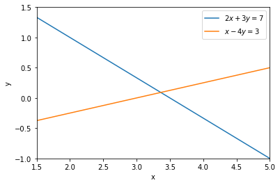
The two lines cross at only one point, at point \( (37/11, 1/11)\). This point is the unique solution of the system, \(\mathbf{x} = (37/11, 1/11)\).
Let’s now consider two systems of two equations whose graphs are parallel lines:
and let us plot them.
x2 = np.linspace(0, 2.5, 10)
y2 = (5 - 2 * x2) / 3

fig, ax = plt.subplots(1, 2, figsize=(10, 4), sharey=True)

ax[0].plot(x1, y1, label=r"$2x + 3y = 7$")
ax[0].plot(x2, y2, label=r"$2x + 3y = 5$")
ax[0].set_aspect('equal')
ax[0].set_xlabel('x')
ax[0].set_ylabel('y')
ax[0].legend(loc='best')

y2 = (14 - 4 * x1) / 6
ax[1].plot(x1, y1, label=r"$2x + 3y = 7$")
ax[1].plot(x1, y2, 'y--', label=r"$4x + 6y = 14$")
ax[1].set_aspect('equal')
ax[1].set_xlabel('x')
ax[1].legend(loc='best')

plt.setp(ax, xlim=(0, 3.7), ylim=(0, 2.5))
plt.show()
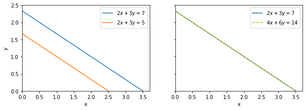
In the first case, the lines never cross because they are parallel. Therefore, the system of equations has no solution. We can write \(\mathbf{x} \in \emptyset\) (empty set).
The lines are parallel in the second case as well, but now they are on top of each other. There are an infinite number of solutions to that system - every point on the line \( y = (7-2x)/3 \) is a solution. We can then write that the solution set is \( \{ (t, \frac{7-2t}{3}), t \in \mathbb{R})\} \).
We can conclude that the existence and uniqueness of the solution of a linear system depends on whether the lines are parallel or not.
Let us test this by finding the cross products of the row-vectors of the coefficient matrices. The row-vectors are normal to the lines given by the equations, so if the equation graphs are parallel, their normals will be too.
from matplotlib.patches import Polygon


x2 = np.linspace(0, 8, 10)
y2 = (x2 - 3) / 4

fig, ax = plt.subplots(1, 2, figsize=(10, 6))

ax[0].plot(x1, y1, label=r"$2x + 3y = 7$")
ax[0].plot(x2, y2, label=r"$x - 4y = 3$")
ax[0].quiver(37/11, 1/11, 2, 3, scale=15, angles='xy', color='b')
ax[0].quiver(37/11, 1/11, 1, -4, scale=15, angles='xy', color='orange')
vertices = np.array([[0, 0], [2, 3], [3, -1], [1, -4]])/4.3 + np.array([37/11, 1/11])
ax[0].add_patch(Polygon(vertices , facecolor='lightblue', alpha=0.7))
ax[0].set_xlim(1.5, 5)
ax[0].set_ylim(-1, 1.5)
ax[0].set_aspect('equal')
ax[0].set_xlabel('x')
ax[0].set_ylabel('y')
ax[0].legend(loc='best')


y2 = (5 - 2 * x2) / 3
ax[1].plot(x1, y1, label=r"$2x + 3y = 7$")
ax[1].plot(x2, y2, label=r"$2x + 3y = 5$")
ax[1].quiver(1.3, 4.4/3, 2, 3, scale=15, angles='xy', color='b')
ax[1].quiver(1.5, 2/3, 2, 3, scale=15, angles='xy', color='orange')
ax[1].set_xlim(0, 3.7)
ax[1].set_ylim(0, 2.5)
ax[1].set_aspect('equal')
ax[1].set_xlabel('x')
ax[1].legend(loc='best')

plt.show()
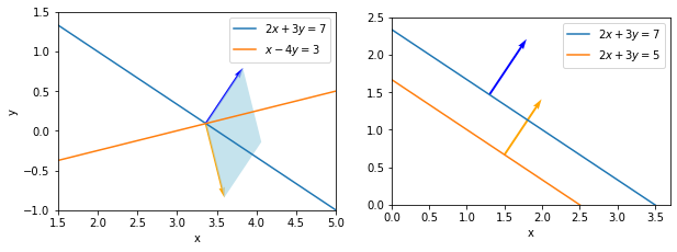
If \(\mathbf{a_1} = (a_{11}, a_{12})\) is the first row-vector of a coefficient matrix and \(\mathbf{a_2} = (a_{21}, a_{22})\), we can express their cross product as:
where \(|\cdot|\) denotes the magnitude of the vector, \(\vartheta\) is the angle between \(\mathbf{a_1}\) and \(\mathbf{a_2}\) and \(\hat{n}\) is the unit normal vector to both vectors. We can see that the magnitude of the vector is equal to the area of a parallelogram with sides \(|\mathbf{u}|\) and \(|\mathbf{v}|\), with \(\vartheta\) controlling how skewed it is. Such a parallelogram is marked by light-blue on the left figure. We also know from the previous notebook that the magnitude of the cross product of the two rows or columns of the matrix is given by the determinant of the matrix:
Let us then conclude, and we will justify this in the next notebooks, that a system of linear equations \(A \mathbf{x} = \mathbf{b}\) will have a unique solution iff \(\det A \neq 0\). If \(\det A = 0\), the system either has infinitely-many solutions or no solutions at all.
Gaussian elimination#
Let us finally formally introduce what we have been trying to achieve in most examples above. Gaussian elimination (or row reduction) uses the three transformations mentioned before to reduce a system to row echelon form. A matrix is in row echelon form if:
all zero rows (if they exist) are below all non-zero rows
the leading coefficient (or pivot; the first non-zero entry in a row) is always strictly to the right of the leading coefficient of the row above it. That is, for two leading elements \(a_{ij}\) and \(a_{kl}\): if \(i < k\) then it is required that \(j < l\).
Notice that these conditions require reduced echelon form to be an upper-trapezoidal matrix. For example:
The motivation behind performing Gaussian elimination is therefore clear, as we have demonstrated in the upper-triangular example why triangular systems are most convenient for solving systems of linear equations.
Let us consider again a general coefficient matrix \(A \in \mathbb{C}^{m \times n}\) in \(A \mathbf{x} = \mathbf{b}\):
What we want to achieve is to have all entries in the 1st column be 0 except for the first one. Then in the 2nd column all entires below the second entry should be 0. In the 3rd column all entries below the third entry should be 0, and so on. That means that we will have to use the 3rd transformation rule and subtract one equation from every one below it, multiplied such that the column entries will cancel:
And so on. Notice that these operations (transformations) are performed on entire rows, so the entries in the entire row change (here denoted by tilde and hat). That is why we need to be careful what row we add to other row since, for example, adding the first row to other rows later on would re-introduce non-zero values in the first column which we previously eliminated.
Example#
Consider the following system of 3 equations and 3 unknowns \(x, y, z\):
Let us write it in augmented-matrix form and perform Gaussian eliminations.
The one transformation on the 3rd equation eliminated both \(x\) and \(y\) unknowns from it so we did not have to perform another transformation. Now the system is reduced to an upper-triangular one, which we have encountered before and know how to solve. We begin from the last equation and back-substitute found values as we work our way up. We leave it to the reader to confirm that there is a unique solution \(\mathbf{x} = (1/3, 2/3, -1/3)\).
Transformations as matrices#
Recall the example on permutations a few notebooks ago, where we wrote each permutation of rows or columns as a permutation matrix multiplying the original matrix. We can do the same thing with elementary row transformations.
Consider the same example from above, where we performed the following 2 transformations on the square \(3 \times 3\) matrix \(A\):
subtracted row 1 from row 2; \(L_2 - L_1 \to L_2\)
added row 1 to row 3; \(L_3 + L_1 \to L_3\)
We can write both of these transformations using elementary matrices:
As in the example of permutations, left-multiplication by an elementary matrix \(E\) represents elementary row operations, while right-multiplication represents elementary column operations. Our transformations are row operations, so we left multiply our original matrix:
resulting in the same upper-triangular matrix as before. Note that the order in which we multiply is, in general, important.
Using the inverse matrix to solve a linear system#
Remember that an inverse of a square matrix \(A\) is \(A^{-1}\) such that \(AA^{-1} = A^{-1}A = I\). Therefore, if we have a matrix equation \(A \mathbf{x} = \mathbf{b}\), finding an inverse \(A^{-1}\) would allow us to solve for all unknowns simultaneously, rather than in steps like in the examples above. Here is the idea:
Finding the solution \(\mathbf{x}\) is then reduced to a matrix-vector multiplication \(A^{-1}\mathbf{b}\).
Gauss-Jordan elimination#
Gauss-Jordan elimination is a type of Gaussian elimination that we can use to find the inverse of a matrix. This process is based on reducing a matrix whose inverse we want to find to reduced row echelon form. For a matrix to be in reduced row echelon form it must satisfy the two conditions written above for row echelon forms and an additional condition:
Each leading (pivot) element is 1 and all other entries in their columns are 0.
Examples of such matrices are:
Now, let \(A \in \mathbb{R}^{n \times n}\) be a square matrix whose inverse we want to find. We use it to form an augmented block matrix \([A | I]\). We perform elementary row transformations on this matrix such that we reduce \(A\) to reduced row echelon form, which we will denote as \(A_R\). In this process, the identity matrix \(I\) on the right will be transformed to some new matrix \(B\). If \(A\) is invertible, we will have:
Let us think why this is. We showed above that elementary row operations can be represented as elementary matrices. Let there be \(k\) such transformations needed to reduce \(A\) to \(A_R\). Then we can write:
and let us denote \(S = E_k E_{k-1} \dots E_2 E_1\), the product of all \(k\) elementary matrices. Now,
Therefore, if \(A_R = I \Rightarrow I = SA\), meaning that \(S = B\) is indeed the inverse of \(A\).
If \(A\) is not invertible, remember that it means that it is not full-rank. What that means is that \(A_R\) will have at least one zero-row. In that case, \(B \neq A^{-1}\).
Example: Calculating an inverse of a matrix#
Let us find the inverse matrix of:
We begin by forming an augmented matrix \([A|I]\) and begin reducing \(A\) to reduced row echelon form.
We successfully found the inverse \(A^{-1} = B\)! Let us now use it to solve the system \(A \mathbf{x} = \mathbf{b}\), where \(\mathbf{b} = (2, 0, 1)^T\). As explained before, \(A\) on the LHS is eliminated by multiplying both sides by \(A^{-1}\) on the left, leaving:
The reader is encouraged to confirm this is the correct solution either through substitution into the original system or by using another solution method.