Chapter 8 – Feedforward
Chapter 8 – Feedforward#
Data Science and Machine Learning for Geoscientists
Let’s take a look at how feedforward is processed in a three layers neural net.
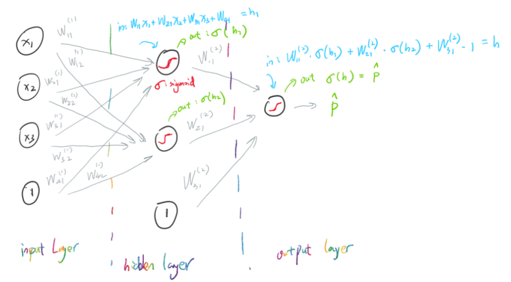 Figure 8.1
From the figure 8.1 above, we know that the two input values for the first and the second neuron in the hidden layer are
where the \(w^{(n)}_{4m}\) term is the bias term in the form of weight.
To simplify the two equations above, we can use matrix
Similarly, the two outputs from the input layer can be the inputs for the hidden layer
This in turns can be the input values for the next layer (output layer)
Again, we can simplify this equation by using matrix
Then we send this value \(h^{(2)}\) into the sigma function in the final output layer to obtain the prediction
To put all the equation of three layers together, we can have
Or we can simplify it to be
This is the feedforward process: based on the known weights \(W\) and input \(x\) to calculate the prediction \(\hat{y}\).
Finally, it’s easy to write code computing the output from a Network instance. We begin by defining the sigmoid function:
def sigmoid(z):
    return 1.0/(1.0+np.exp(-z))
Note that when the input z is a vector or Numpy array, Numpy automatically applies the function sigmoid elementwise, that is, in vectorized form.
We then add a feedforward method to the Network class, which, given an input a for the network, returns the corresponding output:
def feedforward(self, a):
    """Returning the output a, which is the input to the next layer"""
    for b, w in zip(self.biases, self.weights):
        a = sigmoid(np.dot(w, a)+b)
    return a