Stream functions and stream lines

Geophysical Fluid Dynamics of the Oceans

In this notebook, stream functions and streamlines will be explained and visualised.

import numpy as np
import matplotlib.pyplot as plt
import plotly.figure_factory as ff
import plotly.graph_objects as go

A stream function, \(\psi\), is a scalar function of which the derivative gives the velocity field at right angles to the stream function. The stream function is a function of space \((x,y)\) and time and is defined as \(\psi = f(x,y)\).

\[\frac{\partial \psi}{\partial x} = v \]

\[\frac{\partial \psi}{\partial y} = -u \]

where \(u(x,y)\) and \(v(x,y)\) are velocity component functions.

The stream function satisfies the continuity equation and is therefore incompressible. This means that

\[\nabla (u,v) = \frac{\partial u}{\partial x} + \frac{\partial v}{\partial y} = \frac{\partial^2 \psi}{\partial x \partial y} + \frac{\partial^2 \psi}{\partial y \partial x}\]

It can be both rotational and irrotational. It is irrotational if it satisfies Laplace’s equation of the form

\[\frac{\partial^2 \psi}{\partial x^2} + \frac{\partial^2 \psi}{\partial y^2} = 0 \]

Streamlines are the lines along which the stream function is constant, so along a streamline \(d \psi = 0\). A few properties of streamlines are:

• All the streamlines are parallel to each other

• With a constant stream function value, infinite amounts of streamlines can be drawn

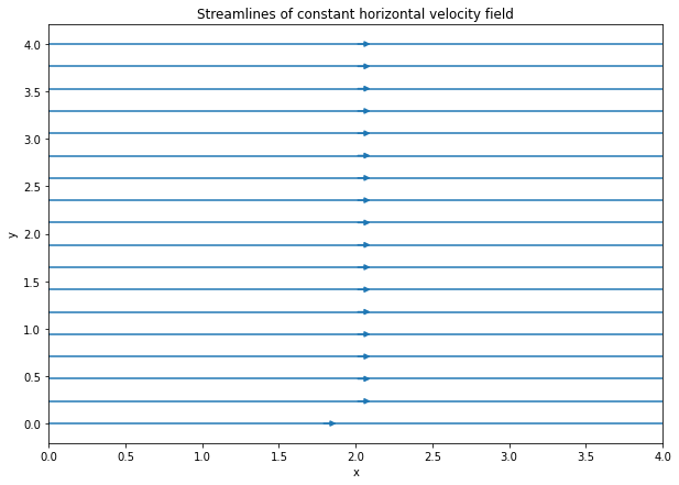
In Python, streamlines can be visualised using the Streamplot within matplotlib that draws the streamlines of a vector field.

# creating a spatial grid
x = np.arange(0, 5)
y = np.arange(0, 5)
X, Y = np.meshgrid(x, y)

# creating components of the velocity field
u = np.ones((5, 5)) # x-component, zeroes
v = np.zeros((5, 5)) # y-component 
 
fig = plt.figure(figsize = (10, 7))
 
plt.title('Streamlines of constant horizontal velocity field')    
plt.xlabel('x')
plt.ylabel('y')
# Plotting stream plot
# density dictates how closely spaced the streamlines are plotted
plt.streamplot(X, Y, u, v, density = 0.6)

<matplotlib.streamplot.StreamplotSet at 0x23ff27a7340>

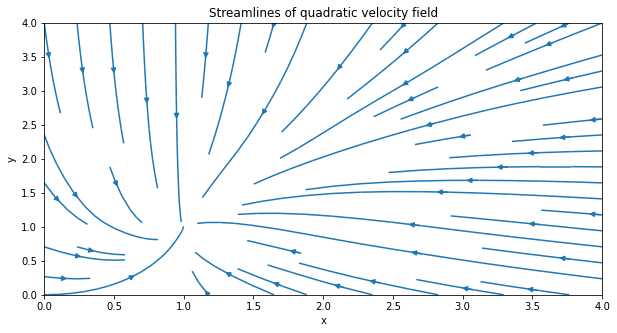
Now, a stream function plot will be made for velocity components that vary within the grid. Now, the x-component of the velocity field, \(u\), will be of the function \(u = 1-x^2\) and the y-component of the field, \(v\), will be defined as \(v = x - y^2\).

x = np.arange(0, 5)
y = np.arange(0, 5)
X, Y = np.meshgrid(x, y)

U = 1 - X**2
V = X - Y**2
 
fig = plt.figure(figsize = (10, 5))
plt.title('Streamlines of quadratic velocity field')    
plt.xlabel('x')
plt.ylabel('y')
plt.streamplot(X, Y, U, V, density = 0.6)

<matplotlib.streamplot.StreamplotSet at 0x23ff2961a60>

A more interactive (move cursor over plot to see coordinates) and other good way to create a stream function plot, is by using figure factory from the Plotly module.

Moreover, a source point can be created using Graph_objects from the Plotly module. Below is shown how this can be plotted. Here, the velocity field \(u\) and y include the source components in their function.

# create spatial meshgrid
x = np.linspace(0, 5, 100)
y = np.linspace(0, 5, 100)
X, Y = np.meshgrid(x, y)

# define source strength and location
source_strength = 10
x_source, y_source = 2, 2

# define velocity field as function X and Y
u = (source_strength *
     (X - x_source)/((X - x_source)**2 + (Y - y_source)**2))
v = (source_strength*
     (Y - y_source)/((X - x_source)**2 + (Y - y_source)**2))

# Create streamline figure
fig = ff.create_streamline(x, y, u, v,
                           name='Stream line')

fig.add_trace(go.Scatter(x=[2], y=[2],
                          mode='markers',
                          marker_size=14,
                          name='Source'))