Superposition of Waves, Reflection and Refraction
Contents
Superposition of Waves, Reflection and Refraction#
In this notebook, wave phases are discussed, as well as superposition, reflection and refraction.
import numpy as np
import matplotlib.pyplot as plt
Phases of waves#
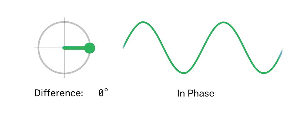
The phase of a wave compared to other waves in superposition or in the group is an important property. Waves for example can have the same function of movement, but can be half a wavelength apart if they are in anti-phase.
It also gives rise to definitions of wavefront, which are contours of joining parts of waves that are all in phase. A ray is perpendicular to that front and dictates the direction of travel.
Superposition of waves#
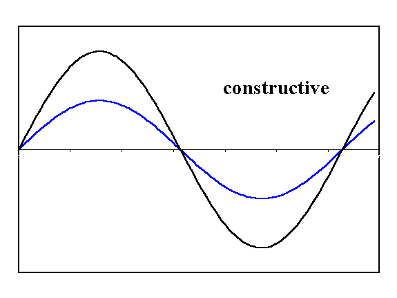
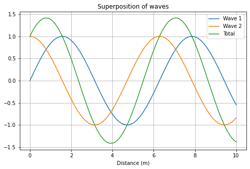
When waves get superimposed, their phase needs to be considered. For example, when waves are exactly \(180\) degrees or \(\pi\) out of phase, destructive interference occurs. If the waves are in phase, constructive interference occurs.
def wave1(y0, k, x):
    return y0 * np.sin(k*x)

def wave2(y0, k, x):
    return y0 * np.sin(k*x + np.pi/2)

x = np.linspace(0, 10, 100)

plt.figure(figsize=(8,5))
plt.xlabel("Distance (m)")
plt.plot(x, wave1(1, 1, x), label = 'Wave 1')
plt.plot(x, wave2(1, 1, x), label = 'Wave 2')
plt.plot(x, wave1(1, 1, x)+wave2(1, 1, x), label = 'Total')
plt.legend()
plt.grid(True)
plt.title("Superposition of waves")
plt.show()
Reflection, refraction and Snell’s law#
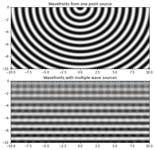
Each point on the wavefront acts as a secondary source of more spherical wavelets.
def function(x,y): return np.sin(2*np.pi*np.sqrt(x**2+y**2))

def wavefront(x,y,pnts=100):
    out=0
    for pt in np.linspace(-20,20,pnts):
        out+=f(x-pt,y,2*np.pi*pt*np.sin(0)) # sin(theta) where theta is 0
    return out

x = np.linspace(-10,10,200)
y = np.linspace(-10,0,200)
X_mesh, Y_mesh = np.meshgrid(x,y)

degree=np.pi/180.

fig=plt.figure()
fig.set_size_inches(8, 8)
ax=fig.add_subplot(2,1,1)
bx=fig.add_subplot(2,1,2)
ax.contourf(X_mesh, Y_mesh, function(X_mesh,Y_mesh), cmap="Greys")
ax.set_title("Wavefronts from one point source", size = "12")
bx.contourf(X_mesh, Y_mesh, wavefront(X_mesh,Y_mesh), cmap="Greys")
bx.scatter(np.linspace(-20,20,100)[25:-25],np.linspace(-20,20,100)[25:-25]*0,cmap="Greys")
bx.set_title("Wavefronts with multiple wave sources", size = "12")
plt.show()
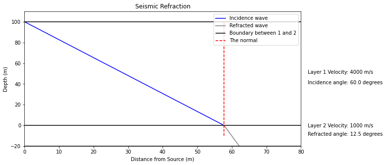
For reflection, the angle of incidence to the normal is the same as the angle of reflection for a wavefront: \(\theta_i = \theta_r\).
Refraction is decribed by Snell’s law. Snell’s law is as follows:
where \(n\) is the ratio of the phase velocity of the two media, also known as the refractive index.

v1 = 4000
v2 = 1000
h = 100 # thickness of layer 1
h2 = 20

fig, ax = plt.subplots(figsize=(10,5))
ax.set_xlabel('Distance from Source (m)')
ax.set_ylabel('Depth (m)')
ax.set_title('Seismic Refraction')

handle = display(None, display_id=True)
bbox = dict(boxstyle ="round", fc = '1')
ax.set_ylim(-h2,h+10)
spacing = 10

# calculate refraction angle, theta_2, from Snell's law
theta_i = np.radians(60)
theta_r = np.arcsin((v2/ v1) * np.sin(theta_i))
theta_s = np.pi/2 - theta_r # angle seen compared to surface instead of normal

# location where incidence wave crosses surface
incidence_wave = (h2-(h+h2))/(-np.tan(incoming_angle))

# plot incidence wave from location x=0 to location of intercept of layers
ax.plot(np.linspace(0,incidence_wave),np.linspace(0,incidence_wave)*-np.tan(theta_i)+h,color='blue', label = 'Incidence wave')
# plot refracted wave from location of intercept to 80m
ax.plot(np.linspace(incidence_wave,80),(np.linspace(incidence_wave,80)-incidence_wave)*-np.tan(theta_s),color='grey', label = 'Refracted wave')
ax.hlines(0,0,80,color='black', label = 'Boundary between 1 and 2') # set horizontal waves indicating layer boundaries
ax.hlines(h,0,80,color='black')
ax.hlines(-h2,0,80,color='black')
ax.vlines(incidence_wave,-10, 100, linestyles = 'dashed', colors = 'red', label = 'The normal')
ax.set_xlim(0,80)
ax.text(82,50,'Layer 1 Velocity: '+str(v1)+' m/s')
ax.text(82,40,'Incidence angle: ' + str(round((theta_i*180/np.pi), 2)) +' degrees')
ax.text(82,-2,'Layer 2 Velocity: '+str(v2)+' m/s')
ax.text(82,-10,'Refracted angle: ' + str(round((theta_r*180/np.pi), 2)) +' degrees')
plt.legend()
None
<matplotlib.legend.Legend at 0x7f831187c4c0>
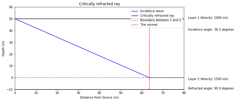
For critically refraced angle, \(\theta_r\) must be \(90\) degrees. A critcally refraced ray travels between the two layers with speed \(v_2\), and is only created when \(v_2 > v_1\).
A head wave forms from the critically refracted ray, since this ray acts as point sources creating semi-circular wavefronts.
v1 = 1000
v2 = 1500
h = 50 # thickness of layer 1
h2 = 10

theta_r = np.radians(90) # critically refraced ray
theta_i = v1/v2
print('For a critically refracted ray, the incidence angle must be',
      str(round((theta_i*180/np.pi),2)), 'degrees')
For a critically refracted ray, the incidence angle must be 38.2 degrees
fig, ax = plt.subplots(figsize=(10,5))

handle = display(None, display_id=True)
bbox = dict(boxstyle ="round", fc = '1')
ax.set_ylim(-h2,h+10)
spacing = 10

# calculate refraction angle, theta_2, from Snell's law
theta_s = np.pi/2 - theta_r # angle seen compared to surface instead of normal

# location where incidence wave crosses surface
incidence_wave = (h2-(h+h2))/(-np.tan(theta_i))

# plot incidence wave from location x=0 to location of intercept of layers
ax.plot(np.linspace(0,incidence_wave),np.linspace(0,incidence_wave)*-np.tan(theta_i)+h,color='blue', label = 'Incidence wave')
# plot refracted wave from location of intercept to 80m
ax.plot(np.linspace(incidence_wave,80),(np.linspace(incidence_wave,80)-incidence_wave)*-np.tan(theta_s),
        color='black', label = 'Critically refracted ray')


ax.hlines(0,0,80,color='grey', linestyles = 'dashed', label = 'Boundary between 1 and 2') # set horizontal waves indicating layer boundaries
ax.hlines(h,0,80,color='black')
ax.hlines(-h2,0,80,color='black')
ax.vlines(incidence_wave,-10, 60, linestyles = 'dashed', colors = 'red', label = 'The normal')
ax.set_xlim(0,80)
ax.text(82,50,'Layer 1 Velocity: '+str(v1)+' m/s')
ax.text(82,40,'Incidence angle: ' + str(round((theta_i*180/np.pi), 2)) +' degrees')
ax.text(82,-2,'Layer 2 Velocity: '+str(v2)+' m/s')
ax.text(82,-10,'Refracted angle: ' + str(round((90.000), 2)) +' degrees')
plt.legend()
ax.set_xlabel('Distance from Source (m)')
ax.set_ylabel('Depth (m)')
ax.set_title('Critically refracted ray')
None
Text(0.5, 1.0, 'Critically refracted ray')