Chapter 6 – Gradient Descent 2
Chapter 6 – Gradient Descent 2#
Data Science and Machine Learning for Geoscientists
Okay, it sounds good in theory so far. But how do we calculate the \(\nabla C\)? Let’s compute the \(\frac{\delta C(\vec{w},b)}{\delta w_1}\) in this 2 layers (input layer and output layer) neural network example.
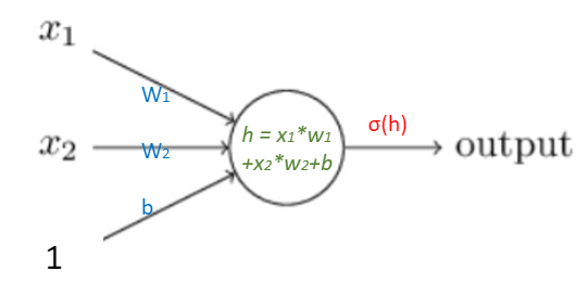 Figure 1.7: Two layer neural network.
It is very easy to write a for loop to compute the sum: from \(y_1\) to \(y_m\), which is summing up the performance of each single individual prediction. So, let’s compute just \(y_i\) for the sake of simplicity. What’s more, the \(y_i\) is just a constant, which we can put it outside of the differential equation, so we have
Let’s look at the first term in the equation (30):
We can break it down so that we can use the chain rule.
According to the chain rule, we have
So the equation (31) becomes
where \(y_i\) is the actual result and \(\hat{y}\) is the predicted result by the AI.
Similarly, we can do the same for the second term in equation (30) and have the combined result as follow
Again, do not forget that we ignored the summation symbol \(\sum\) for simplicity before. So the actual result of the gradient of the loss/cost function is
This is actually a very neat result. How do we interpret it? Well, the gradient of the cost function of any single neuron, which has weight \(w_i\), is evaluated by the difference between the predicted and actual \(y\) values for all students or data (i.e. the error). The larger the error, the faster the neuron will learn. This is just what we’d intuitively expect. It is also related to the input \(x\) values of that particular neuron.
Anyway, in order to update the weight \(w_i\) as derived earlier in the previous chapter in equation (27), we just need to plug in \(\frac{\delta C}{\delta w_i}\), which we just obtained.
It is the same mathematical process for updating the bias term \(b\), we will just write down the result here