Pourbaix Diagram#

Low-Temperature Geochemistry

# import relevant modules

%matplotlib inline
import numpy as np
import matplotlib.pyplot as plt

In this session, we will see how pourbaix diagrams (\(pe\)-\(pH\) dominance diagrams) are made and how to read and interpret them.

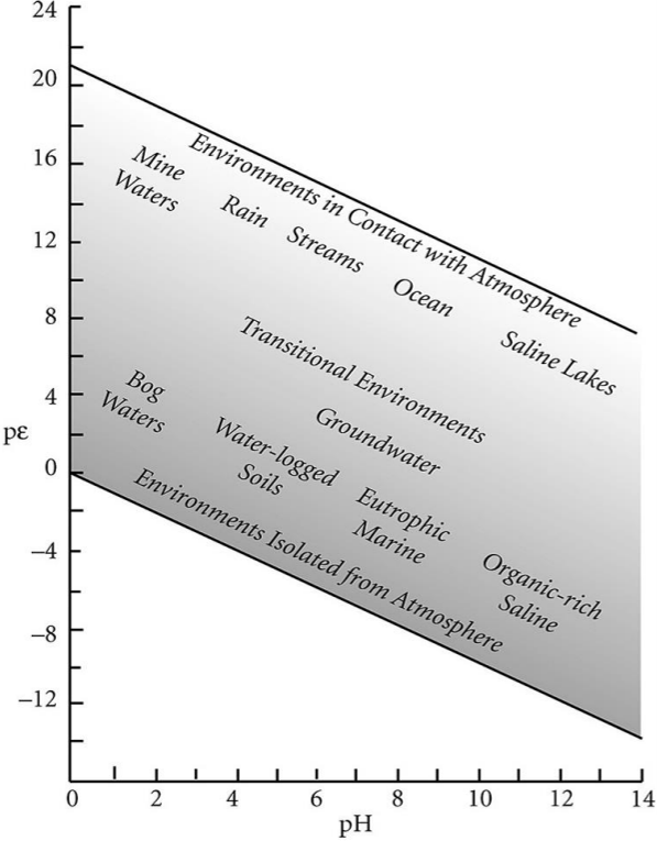
Pourbai diagrams show which species predominates in given \(pe\)-\(pH\) regions, i.e., the dominant species varies as a function of \(pe\) (i.e. mostly oxygen) and \(pH\) This affects the distribution and transport of elements in the world! The diagrams can also be applied to

Types of ores/minerals which are related to the environmental conditions when they were formed
Ore recovery
Pollutant transport
Elemental budgets
Batteries
Ecology
etc.

Consider a generic “half cell” reduction reaction including \(H^+\):

\[Ox + n_e \cdot (e^-) + n_{H} \cdot H^+ = Red\]

The equlibrium constant of this half-reaction can be written as:

\[K = \frac{a_{Red}}{a_{Ox} \cdot a_{e^-}^{n_e} \cdot a_{H^+}^{n_H}}\]

Recall Nernst’s equation:

\[E_{cell} = E_{cell}^o - \frac{RT}{n_e \cdot F} \ln Q\]

and the relationship between the Gibbs free energy (\(\Delta G\)) and \(E_{cell}\) of a redox reaction:

\[\Delta G = -n_eFE_{cell}\]

At equilibrium, \(Q = K\) and \(E_{cell} = 0\), so from the two equations we can derive the relationship between the equilibrium constant and standard voltage potential:

\[\ln K = \frac{n_e \cdot F}{RT}\cdot E_{cell}^o\]

We are considering a reaction coupled with the hydrogen electrode, so \(E_{cell}^o = E_{h}^o\).

Substituting \(K\) of this half-reaction, we get:

\[\ln \left(\frac{a_{Red}}{a_{Ox} \cdot a_{e^-}^{n_e} \cdot a_{H^+}^{n_H}}\right) = \frac{n_e \cdot F}{RT}\cdot E_{h}^o\]

\[\log \left(\frac{a_{Red}}{a_{Ox} \cdot a_{e^-}^{n_e} \cdot a_{H^+}^{n_H}}\right) = \frac{n_e \cdot F}{2.303 RT}\cdot E_{h}^o\]

\[\log \left(\frac{a_{Red}}{a_{Ox}} \cdot \frac{1}{a_{e^-}^{n_e}} \cdot \frac{1}{a_{H^+}^{n_H}}\right) = \frac{n_e \cdot F}{2.303 RT}\cdot E_{h}^o\]

\[\log \left(\frac{a_{Red}}{a_{Ox}}\right) - n_e \log(a_{e^-}) - n_H \log(a_{H^+}) = \frac{n_e \cdot F}{2.303 RT}\cdot E_{h}^o\]

By definition of \(p\) (e.g. \(pH = -\log a_{H^+}\)),

\[\log \left(\frac{a_{Red}}{a_{Ox}}\right) + n_e pe + n_H pH = \frac{n_e \cdot F}{2.303 RT}\cdot E_{h}^o\]

Dividing by \(n_e\), we get:

\[\frac{1}{n_e} \log \left(\frac{a_{Red}}{a_{Ox}}\right) + pe + \frac{n_H}{n_e} pH = \frac{F}{2.303 RT}\cdot E_{h}^o\]

Recall from the lecture slide that \(pe^o = \frac{F}{2.303 RT}\cdot E_{h}^o\), so

\[\frac{1}{n_e} \log \left(\frac{a_{Red}}{a_{Ox}}\right) + pe + \frac{n_H}{n_e} pH = pe^o\]

\[pe = pe^o - \frac{1}{n_e} \log \left(\frac{a_{Red}}{a_{Ox}}\right) - \frac{n_H}{n_e} pH\]

If \(a_{Red} = a_{Ox}\), then:

\[pe = pe^o - \frac{n_H}{n_e} pH\]

which is a boundary (where the activities of two species are equal) in pourbaix diagrams. It is a linear equation (\(pe\) vs. \(pH\)) with slope = \(- \frac{n_H}{n_e}\) and y-intercept = \(pe^o\).

Next, we will consider the upper and lower limits of water in a pourbaix diagram.

(1) Consider the reduction of oxygen into water:

\[\frac{1}{2}O_2 + 2 \cdot (e^-) + 2 \cdot H^+ = H_2O \quad ; \quad pe^o = 20.75\]

After some manipulations similar to the above, we get:

\[pe = pe^o - \log \left(\frac{a_{H_2O}}{a_{O_2}^{0.5}}\right) - pH\]

\[pe = pe^o - \log(a_{H_2O}) + \frac{1}{2}\log(a_{O_2}) - pH\]

\[pe = pe^o + \frac{1}{2}\log(a_{O_2}) - pH\]

\[pe = pe^o + \frac{1}{2}\log(P_{O_2}) - pH\]

\(1\,atm\) is the maximum pressure in the atmosphere today, so we will assign \(P_{O_2} = 1\) (Actual \(P_{O_2} = 0.21\,atm\)), and \(pe^o = 20.75\)

\[\therefore pe = 20.75 - pH\]

is the equation representing the upper limit.

(2) Consider the reduction of hydrogen:

\[1 \cdot (e^-) + 1 \cdot H^+ = \frac{1}{2}H_2 \quad ; \quad pe^o = 0\]

After some manipulations similar to the above, we get:

\[pe = pe^o - \frac{1}{2}\log(a_{H_2}) - pH\]

\(1\,atm\) is the maximum pressure in the atmosphere today, so we will assign \(P_{H_2} = 1\), and \(pe^o = 20.75\)

\[\therefore pe = - pH\]

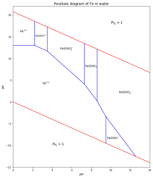
If we want to create a pourbaix diagram of an element in our environment, we need to have the information about all half-reactions involved. The plot below is the pourbaix diagram of \(Fe\)-\(H_2O\) system.

# name each ion by easy characters
# 3A = Fe^{3+}, 3B = Fe(OH)^{2+}, 3C = Fe(OH)_2^+, 3D = Fe(OH)_3, 3E = Fe(OH)_4^-  # Fe oxidation number = +3
# 2A= Fe^{2+}, 2B = Fe(OH)^-  # Fe oxidation number = +2

# pe-pH equations of each boundary - taken from https://slideplayer.com/slide/14759609/
# vertical boundaries
pH_3A_3B = 2.2
pH_3B_3C = 3.5
pH_3C_3D = 7.3
pH_3D_3E = 8.6
pH_2A_2B = 9.5
# horizontal and inclined boundaries
def pe_3A_2A(pH): return 13.0
def pe_3B_2A(pH): return 15.2 - pH
def pe_3C_2A(pH): return 18.7 - 2*pH
def pe_3D_2A(pH): return 26 - 3*pH
def pe_3E_2B(pH): return 25.1 - 3*pH
def pe_reduction_of_O(pH): return 20.75 - pH
def pe_reduction_of_H(pH): return - pH

# plot boundaries
plt.figure(figsize=(10,12)) # set figure
pH_range = [0, 14]
plt.plot(pH_range, pe_reduction_of_O(np.array(pH_range)) , 'r')  # upper stability limit of water
plt.plot(pH_range, pe_reduction_of_H(np.array(pH_range)) , 'r')  # lower stability limit of water
plt.plot([0, pH_3A_3B], [pe_3A_2A(0), pe_3A_2A(pH_3A_3B)], 'b')  # 3A-2A
plt.plot([pH_3A_3B, pH_3A_3B], [pe_3A_2A(pH_3A_3B), pe_reduction_of_O(pH_3A_3B)], 'b')  # 3A-3B
plt.plot([pH_3A_3B, pH_3B_3C], [pe_3B_2A(pH_3A_3B), pe_3B_2A(pH_3B_3C)], 'b')  # 3B-2A
plt.plot([pH_3B_3C, pH_3B_3C], [pe_3B_2A(pH_3B_3C), pe_reduction_of_O(pH_3B_3C)], 'b')  # 3B-3C
plt.plot([pH_3B_3C, pH_3C_3D], [pe_3C_2A(pH_3B_3C), pe_3C_2A(pH_3C_3D)], 'b')  # 3C-2A
plt.plot([pH_3C_3D, pH_3C_3D], [pe_3C_2A(pH_3C_3D), pe_reduction_of_O(pH_3C_3D)], 'b')  # 3C-3D
plt.plot([pH_3C_3D, pH_3D_3E], [pe_3D_2A(pH_3C_3D), pe_3D_2A(pH_3D_3E)], 'b')  # 3D-2A
plt.plot([pH_3D_3E, pH_3D_3E], [pe_3D_2A(pH_3D_3E), pe_reduction_of_O(pH_3D_3E)], 'b')  # 3D-3E
plt.plot([pH_2A_2B, pH_2A_2B], [pe_3E_2B(pH_2A_2B), pe_reduction_of_H(pH_2A_2B)], 'b')  # 2A-2B
plt.plot([pH_2A_2B, 12.55], [pe_3E_2B(pH_2A_2B), pe_3E_2B(12.55)], 'b')  # 3E-2B  # pH=12.55 is where pe_reduction_of_H = pe_3E_2B
plt.plot([pH_3D_3E, pH_2A_2B], [pe_3D_2A(pH_3D_3E), pe_3E_2B(pH_2A_2B)], 'b')  # 3D-2A
# label and title the plot
plt.xlabel('$pH$', fontsize=12)
plt.ylabel('$pe$', fontsize=12)
plt.xlim(pH_range)
plt.ylim([-15, 22])
plt.title('Pourbaix diagram of $Fe$ in water', fontsize=14)
# label each stability regions
plt.text(0.7, 16, '$Fe^{3+}$', fontsize=12)
plt.text(2.25, 15, '$Fe(OH)^{2+}$', fontsize=10)
plt.text(4.8, 12, '$Fe(OH)_2^+$', fontsize=12)
plt.text(7.35, 8, '$Fe(OH)_3$', fontsize=12)
plt.text(10.8, 2, '$Fe(OH)_4^-$', fontsize=12)
plt.text(3, 4, '$Fe^{3+}$', fontsize=12)
plt.text(9.6, -8.5, '$Fe(OH)^-$', fontsize=12)
plt.text(10, 18, '$P_{O_2}>1$', fontsize=14)
plt.text(4, -10, '$P_{H_2}>1$', fontsize=14)

Text(4, -10, '$P_{H_2}>1$')

References#

Farmer, M. (2019) GEOCHEMICAL METHODS FOR THE DETERMINATION OF DIFFERENT METAL SPECIES. https://slideplayer.com/slide/14759609/. (Accessed 28 September 2022).
Lecture slide for Lecture 5 of the Low-Temperature Geochemistry module

ESE Jupyter Material

Pourbaix Diagram

Contents

Pourbaix Diagram#

References#