Wave equation

Mathematics for Scientists and Engineers 2

Finally we consider a hyperbolic PDE: the simple wave equation

\[ u_{tt} = c^2 \nabla^2 u \]

where \( u \) is the displacement of the string. Since the wave equation is second order in time, we will require two initial conditions. We can also write it using the d’Alembert (or box) operator \( \Box \equiv \frac{1}{c^2} \partial_{tt} - \nabla^2 \) as \( \Box u = 0 \).

Physical interpretation

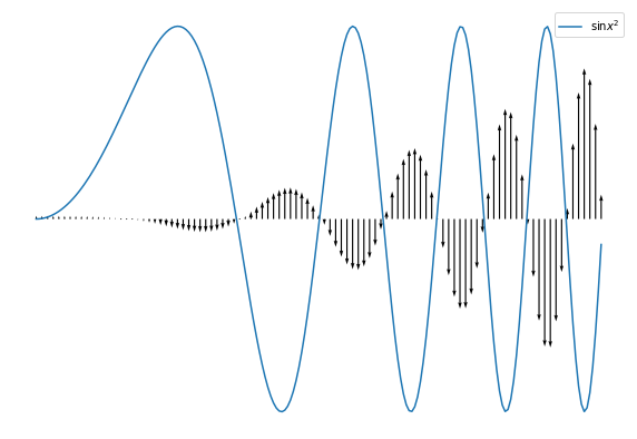
Since \( u \) represents displacement of the string, then \( u_{tt} \) is the acceleration of a point due to tension. So the acceleration of a point is proportional to the concavity at the point, which is related to \( \nabla^2 \) - the larger the concavity, the larger the acceleration is.

import numpy as np
import matplotlib.pyplot as plt


x = np.linspace(0, 5, 201)

u = np.sin(x**2)
u_xx = 2*np.cos(x**2) - 4*x**2*np.sin(x**2)
u_xx /= u_xx.max()

fig = plt.figure(figsize=(10, 7))
ax = fig.add_subplot(111)

ax.plot(x, u, label=r'$\sin x^2$')
ax.quiver(x[::2], u[::2]*0, 0, u_xx[::2], units='xy', width=0.01)

ax.legend(loc='best')
ax.axis('off')
plt.show()

D’Alembert’s formula

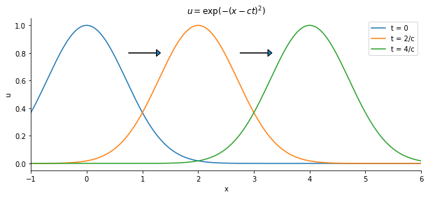
We showed in a previous notebook that the general solution of the 1 + 1-D wave equation \( u_{tt} = c^2 u_{xx} \) can always be written in the form

\[ u(t, x) = f(x - ct) + g(x + ct) \]

What this tells us is that every solution of the wave equations consists of two parts: one moving in the positive x-direction and the other in the negative x-direction, both with velocity \( c \).

x = np.linspace(-2, 8, 201)

u0 = np.exp(-x**2)
u1 = np.exp(-(x-2)**2)
u2 = np.exp(-(x-4)**2)

fig = plt.figure(figsize=(10, 4))
ax = fig.add_subplot(111)

ax.plot(x, u0, label='t = 0')
ax.plot(x, u1, label='t = 2/c')
ax.plot(x, u2, label='t = 4/c')

ax.arrow(0.75, 0.8, 0.5, 0, head_width=0.05)
ax.arrow(2.75, 0.8, 0.5, 0, head_width=0.05)

ax.set_title(r'$u = \exp (- (x-ct)^2)$')
ax.set_xlabel('x')
ax.set_ylabel('u')

ax.set_xlim(-1, 6)
ax.legend(loc='best')
ax.spines['right'].set_visible(False)
ax.spines['top'].set_visible(False)

plt.show()

Now consider an infinite string and two general initial conditions, the first for initial displacement \( u \) and the second for initial vertical velocity \( u_t \):

\[\begin{split} u(0, x) = h(x) \\ u_t(0, x) = v(x) \end{split}\]

As we would with ODEs, we substitute our general solution into these:

\[\begin{split} u(0, x) = f(x) + g(x) = h(x) \\ u_t(0, x) = -c f' (x) + c g' (x) = v(x) \end{split}\]

We divide by \( c \) and integrate the second equation along \( x \) coordinate:

\[ -f + g + K = \frac{1}{c} \int_{x_0}^{x} v(s) \ ds \]

where \( K = f(x_0) - g(x_0) \). So we have a system of two equations:

\[\begin{split} f(x) + g(x) = h(x) \\ -f(x) + g(x) = -K + \frac{1}{c} \int_{x_0}^{x} v(s) \ ds \end{split}\]

Which we easily solve for \( f \) and \( g \):

\[\begin{split} f(x) = \frac{1}{2} \big( h(x) + K \big) - \frac{1}{2c} \int_{x_0}^x v(s) \ ds \\ g(x) = \frac{1}{2} \big( h(x) - K \big) + \frac{1}{2c} \int_{x_0}^x v(s) \ ds \end{split}\]

So the solution is

\[\begin{split} \begin{aligned} u(t, x) &= f(x-ct) + g(x+ct) \\ &= \frac{1}{2} \big( h(x-ct) + K \big) - \frac{1}{2c} \int_{x_0}^{x-ct} v(s) \ ds + \frac{1}{2} \big( h(x+ct) - K \big) + \frac{1}{2c} \int_{x_0}^{x+ct} v(s) \ ds \end{aligned} \end{split}\]

Which we tidy up to get the d’Alembert’s formula:

\[ u(t, x) = \frac{1}{2} \big( h(x-ct) + h(x+ct) \big) + \frac{1}{2c} \int_{x-ct}^{x+ct} v(s) \ ds \]

Example

Farlow 1993, p.135, problem 3: What is the solution to the initial-value problem

\[\begin{split} \begin{aligned} & u_{tt} = u_{xx}, \qquad -\infty < x < \infty, 0 < t < \infty \\ & u(0, x) = \exp(-x^2) \\ & u_t(0, x) = 0 \end{aligned} \end{split}\]

Following the d’Alembert’s formula, we find that the solution is

\[ u(t, x) = \frac{1}{2} \big( e^{-(x-t)^2} + e^{-(x+t)^2} \big) \]

import matplotlib.animation as animation
from IPython.display import HTML


def u(t, x):
    return 0.5 * (np.exp(-(x-t)**2) + np.exp(-(x+t)**2))


x = np.linspace(-5, 5, 201)
yy = [u(i*0.05, x) for i in range(151)]

fig = plt.figure(figsize=(8, 4))
ax = fig.add_subplot(111)

def animate(i):
    ax.clear()
    ax.plot(x,yy[i])
    ax.set_xlim((-5, 5))
    ax.set_ylim((0, 1))
    ax.set_xlabel('x')
    ax.set_ylabel('u')
    ax.set_title(f't = {i*0.05:.2f}')
    ax.grid(True)
    
    
anim = animation.FuncAnimation(fig,animate,frames=150,interval=30)
plt.show()

HTML(anim.to_html5_video())

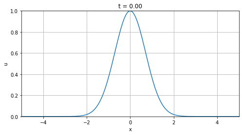
Notice that, as we mentioned earlier, we have two parts: one moving to the left and one to the right with speed \( c = 1 \).