Introduction to Modelling

Mathematics Methods 1

# This cell just imports relevant modules

import numpy as np
import scipy
import scipy.interpolate as si
import scipy.optimize as optimize
from math import pi, exp
import matplotlib.pyplot as plt

Numerical differentiation

Slide 16

Computing first derivatives using central differences

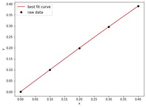
x = np.array([0.0, 0.1, 0.2, 0.3, 0.4])
y = np.array([0.0, 0.0998, 0.1987, 0.2955, 0.3894])

# Here, the argument value of 0.1 is the 'sample distance' (i.e. dx)
derivatives = np.gradient(y, 0.1)
for i in range(0, len(x)):
    print("The derivative at x = %f is %f" % (x[i], derivatives[i])) 

The derivative at x = 0.000000 is 0.998000
The derivative at x = 0.100000 is 0.993500
The derivative at x = 0.200000 is 0.978500
The derivative at x = 0.300000 is 0.953500
The derivative at x = 0.400000 is 0.939000

lp = si.lagrange(x, y)

xi = np.linspace(0, 0.4, 100)

fig = plt.figure(figsize=(8,6))
plt.plot(xi, lp(xi), 'r', label='best fit curve')
plt.plot(x, y, 'ko', label='raw data')
plt.xlabel('x')
plt.ylabel('y')
plt.legend(loc='best', fontsize=12)

plt.show()

Numerical integration

Slide 32

time = np.array([0, 1, 2, 3, 4, 5, 6]) # Time in hours
discharge = np.array([0.07, 0.1, 0.06, 0.02, 0.07, 0.06, 0.05]) # Flow rate in m**3/s
time = time*3600.0 # Convert time in hours into time in seconds

integral = np.trapz(discharge, x=time) # Integrate using the trapezoidal rule. Units are m**3
print("The integral of the discharge data w.r.t. time is %.d m3" % integral) 

The integral of the discharge data w.r.t. time is 1332 m3

t = np.ones((len(time), 2))
for i in range(len(time)):
    t[i] = t[i] * i
    
t = t * 3600
    
y = np.zeros((len(discharge), 2))
for i in range(len(discharge)):
    y[i][1] = discharge[i]

fig = plt.figure(figsize=(8,6))

plt.plot(time, discharge, 'r', label='discharge over time')
plt.plot(time, discharge, 'bo', label='raw data')
for i in range(len(t)):
    plt.plot(t[i], y[i], 'k')
plt.xlabel('time (s)')
plt.ylabel('discharge (m3/s)')
plt.legend(loc='best', fontsize=12)
plt.title('Discharge over time', fontsize=14)
plt.ylim(0, 0.11)

plt.show()

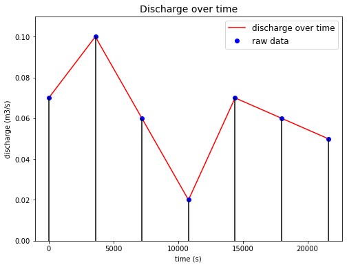
area = 0
dt = 3600
for i in range(1,len(time)):
    area += 0.5 * (discharge[i]+discharge[i-1]) * dt
    
print("Area under all trapeziums =", area, "m3")

Area under all trapeziums = 1332.0 m3

Forward Euler Method

Slide 80

print("Applying the forward Euler method to solve: dy/dx = 2*x*(1-y)...") 
def derivative(x,y):
    return 2*x*(1-y)

n = 7 # Number of desired solution points
dx = 0.4 # Distance between consecutive solution points along the x axis

x = np.zeros(n) # x value at each solution point, initially full of zeros.
y = np.zeros(n) # y value at each solution point, initially full of zeros.

# Now set up the initial condition. These two lines aren't really needed 
# since we have already initialised each component of the array to zero,
# but we'll put them here for completeness.
x[0] = 0
y[0] = 0 
print(f"At x = {x[0]}, y = {y[0]}")  # Print out the initial condition

for i in range(0, n-1):
    x[i+1] = x[i] + dx
    y[i+1] = y[i] + derivative(x[i],y[i])*dx
    print(f"At x = {x[i+1]:.1f}, y = {y[i+1]:.1f}") 

Applying the forward Euler method to solve: dy/dx = 2*x*(1-y)...
At x = 0.0, y = 0.0
At x = 0.4, y = 0.0
At x = 0.8, y = 0.3
At x = 1.2, y = 0.8
At x = 1.6, y = 1.0
At x = 2.0, y = 1.0
At x = 2.4, y = 1.0

xi = np.linspace(0, 2.4, 100)
yi = 1 - np.exp(-xi**2)

fig = plt.figure(figsize=(16,6))

ax1 = fig.add_subplot(121)
ax1.plot(x, y, 'r')
ax1.set_xlabel('x')
ax1.set_ylabel('y(x)')
ax1.set_title("Solution to ODE from forward Euler method", fontsize=14)
ax1.grid(True)

ax2 = fig.add_subplot(122)
ax2.plot(xi, yi, 'b')
ax2.set_xlabel('x')
ax2.set_ylabel('y(x)')
ax2.set_title("Analytical solution to ODE", fontsize=14)
ax2.grid(True)

plt.show()

Root finding

Bisection method

Slide 83

Finding the root using bisection method in Python using scipy.optimize.bisect

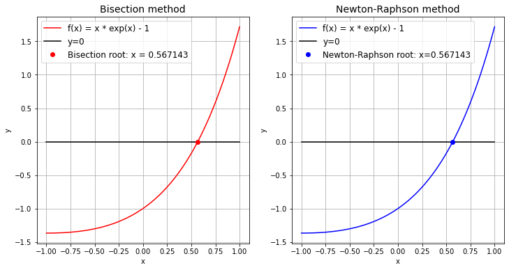
def f(x):
    return x*exp(x) - 1

# We must specify limits a and b in the arguments list
# so the method can find the root somewhere in between them.
bisect_root = optimize.bisect(f, a=0, b=1)

# Print out the root. Also print out the value of f at the root, 
# which should be zero if the root has been found accurately.
print(f"The root of the function f(x) is: {bisect_root:.6f}. At this point, f(x) = {f(bisect_root):.6f}") 

The root of the function f(x) is: 0.567143. At this point, f(x) = 0.000000

Newton-Raphson method

Slide 114

Finding the root using Newton-Raphson method in Python using scipy.optimize.newton

def f(x):
    return x*exp(x) - 1

# We must provide the method with a starting point x0 (here we have chosen x0=0).
newton_root = optimize.newton(f, x0=0)
print(f"The root of the function f(x) is: {newton_root:.6f}. At this point, f(x) = {f(newton_root):.6f}") 

The root of the function f(x) is: 0.567143. At this point, f(x) = -0.000000

if np.allclose(bisect_root, newton_root) == True:
    print("Roots obtained from bisection and Newton-Raphson methods are the same")
else:
    print("Roots obtained from bisection and Newton-Raphson methods are NOT the same")

x = np.linspace(-1, 1, 100)
y = x * np.exp(x) - 1
yi = np.zeros(len(x))

fig = plt.figure(figsize=(12,6))

ax1 = fig.add_subplot(121)
ax1.plot(x, y, 'r', label='f(x) = x * exp(x) - 1')
ax1.plot(x, yi, 'k', label='y=0')
ax1.plot(bisect_root, f(bisect_root), 'ro', label='Bisection root: x = %.6f' % (bisect_root))
ax1.set_xlabel('x')
ax1.set_ylabel('y')
ax1.set_title('Bisection method', fontsize=14)
ax1.legend(loc='best', fontsize=12)
ax1.grid(True)

ax2 = fig.add_subplot(122)
ax2.plot(x, y, 'b', label='f(x) = x * exp(x) - 1')
ax2.plot(x, yi, 'k', label='y=0')
ax2.plot(newton_root, f(newton_root), 'bo', label='Newton-Raphson root: x=%.6f' % (newton_root))
ax2.set_xlabel('x')
ax2.set_ylabel('y')
ax2.set_title('Newton-Raphson method', fontsize=14)
ax2.legend(loc='best', fontsize=12)
ax2.grid(True)

plt.show()

Roots obtained from bisection and Newton-Raphson methods are the same

Dominant eigenvalues

Slide 156

Find dominant eigenvalues in Python using numpy.linalg.eigvals

A = np.array([[2, 2],
              [1, 4]])

print("The eigenvalues of A are %.f and %.f" % (np.linalg.eigvals(A)[0], np.linalg.eigvals(A)[1]))

# The max and abs functions have been used to pick out the eigenvalue with the largest magnitude.
print("The dominant eigenvalue of A is: %.f" % max(abs(np.linalg.eigvals(A)))) 

The eigenvalues of A are 1 and 5
The dominant eigenvalue of A is: 5

Note

Note that for sparse matrices, we can use the following scipy function. The optional argument k is for controlling the desired number of eigenvalues returned.

print(scipy.sparse.linalg.eigs(A, k=1)) 

(array([1.26794919+0.j, 4.73205081+0.j]), array([[-0.9390708 , -0.59069049],
       [ 0.34372377, -0.80689822]]))

C:\Users\Dundo\Anaconda3\lib\site-packages\scipy\sparse\linalg\eigen\arpack\arpack.py:1269: RuntimeWarning: k >= N - 1 for N * N square matrix. Attempting to use scipy.linalg.eig instead.
  RuntimeWarning)