CO2-H2O System
Contents
CO2-H2O System#
In this session, we will derive the governing equations of the \(CO_2\)-\(H_2O\) system under closed and open system conditions.
# import relevant modules

%matplotlib inline
import numpy as np
import matplotlib.pyplot as plt
import pandas as pd
from IPython.display import display
%%javascript
MathJax.Hub.Config({
    TeX: { equationNumbers: { autoNumber: "AMS" } }
});
MathJax.Hub.Queue(
  ["resetEquationNumbers", MathJax.InputJax.TeX],
  ["PreProcess", MathJax.Hub],
  ["Reprocess", MathJax.Hub]
);
Consider the dissociation of a weak poly-protic acid (\(H_2CO_3\)) in water at \(25^\circ C\) and an atmospheric pressure of \(1\) bar.
(1) \(H_2CO_3\) dissociates to form hydrogen ions (\(H^+\)) and bicarbonate ions (\(HCO_{3}^{-}\))
(2) \(HCO_{3}^{-}\) dissociates to form hydrogen ions and carbonate ions (\(CO_{3}^{2-}\))
(3) Dissociation of water
(4) Charge balance (all solutions are electrically neutral). Note that we need to balance concentrations (\(m\)), not activities (\(a\)), as concentrations represent actual quantities of ions.
Now we have \(5\) unknowns (\(m_{H^+}, m_{H_2CO_3}, m_{HCO_{3}^{-}}, m_{CO_{3}^{2-}}, m_{OH^-}\)) but only \(4\) equations. We need the fifth equation in order to solve the simultaneous equations. Fortunately, we can get it from the boundary conditions, i.e. what we know about the system.
For a closed system, the boundary condition is that the total amount of \(CO_2\) in the system is fixed. As \(H_2CO_3\), \(HCO_{3}^{-}\), and \(CO_{3}^{2-}\) form when \(CO_2\) dissolves in water, so
Recalling the relationship between concentration and activity:
We will assume that \(y_{H_2CO_3} = y_{HCO_{3}^{-}} = y_{CO_{3}^{2-}} = y_{OH^-} = 1\), so \(m_i = a_i\).
And recall that
From (294), \(m_{H^+}=10^{-pH}\), rearranging it and using the assumption, we get:
From \(m_{H^+}=10^{-pH}\), (310) and (299), using the assumption, we get:
Substituting (299) and (300) into (298), we get:
We will define a new parameter \(F_H\) as
So,
Substituting (301) into (299) and (300), we get:
The derivations of (301), (302) and (303) lead to the speciation of the carbon system as a function of \(pH\), as shown below.
# function for calculating F_H, m_H2CO3, m_HCO3-, m_CO3--, m_H+, m_OH-
def FH(pH):
    K1 = 10**-6.35
    K2 = 10**-10.33
    return 1+(K1/(10**-pH))+(K2*K1/(10**(-2*pH)))

def m_H2CO3(m_total, pH):
    return m_total/FH(pH)

def m_HCO3(m_total, pH):
    K1 = 10**-6.35
    return m_total*K1/(FH(pH)*(10**-pH))

def m_CO3(m_total, pH):
    K1 = 10**-6.35
    K2 = 10**-10.33
    return m_total*K2*K1/(FH(pH)*(10**(-2*pH)))

def m_H(pH):
    return 10**-pH

def m_OH(pH):
    return 10**-(14-pH)

# plot
plt.figure(figsize=(8,6))
m_total = 0.01  # set m_total value
pH = np.linspace(1, 13, 100)
plt.plot(pH, m_H2CO3(m_total, pH), 'r', label='$H_2CO_3$')  # H2CO3
plt.plot(pH, m_HCO3(m_total, pH), 'g', label='$HCO_{3}^{-}$')  # HCO3-
plt.plot(pH, m_CO3(m_total, pH), 'b', label='$CO_{3}^{2-}$')  # CO3--
plt.plot(pH, m_H(pH), '#FFB53C', label='$H^+$')  # H+
plt.plot(pH, m_OH(pH), '#3CF0FF', label='$OH^-$')  # OH-
plt.plot(6.35, m_H2CO3(m_total, 6.35), 'ko')  # the point where m_H2CO3=m_HCO3-
plt.plot([6.35, 6.35], [0, m_H2CO3(m_total, 6.35)], 'k:')
plt.text(5.5, 0.015, '$pH=6.35$', fontsize=14)
plt.plot(10.33, m_HCO3(m_total, 10.33), 'ko')  # the point where m_HCO3-=m_CO3--
plt.plot([10.33, 10.33], [0, m_HCO3(m_total, 10.33)], 'k:')
plt.text(9.4, 0.015, '$pH=10.33$', fontsize=14)
plt.xlabel('$pH$')
plt.ylabel('Activity $(mol/kg)$')
plt.xlim([1, 13])
plt.ylim([10**-8, 1])
plt.yscale("log")
plt.title('Speciation of the carbon system as a function of pH', fontsize=14)
plt.legend(loc='best', fontsize=10)
<matplotlib.legend.Legend at 0x1fd60a9e460>
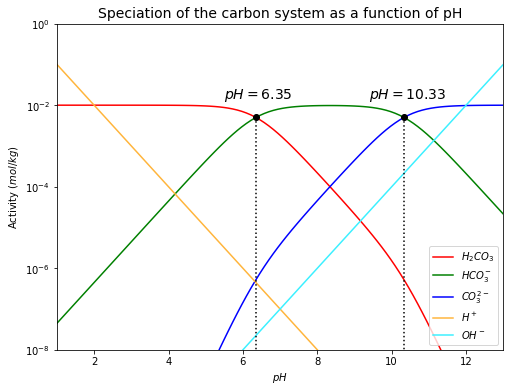
From the plot above, it can be seen that there are two points where the concentrations (activities) of two carbon-bearing species are equal.
\(m_{H_2CO_3} = m_{HCO_{3}^{-}}\)
\(\quad\)If \(m_{H_2CO_3} = m_{HCO_{3}^{-}}\), so
\(m_{HCO_{3}^{-}} = m_{CO_{3}^{2-}}\)
\(\quad\)If \(m_{HCO_{3}^{-}} = m_{CO_{3}^{2-}}\), so
Next, we will consider an open system at \(25^\circ C\) and an atmospheric pressure of \(1\) bar with a constant atmospheric partial pressure of \(CO_2\) (\(pCO_2\))
Some \(CO_2\) in the air will dissolve in water. The amount of dissolved \(CO_2\) follows Henry’s law.
Some dissolved \(CO_2\) will react with water to form carbonic acid:
Rearranging (304) and (305), we get:
Substituting (306) into (307), we get:
Combine both of the carbon-bearing species in water as \(H_2CO_3^*\)
In reality, \(K_H >> K_0\), so \(a_{(CO_2)_{aq}} >> a_{H_2CO_3}\), and
Recall (294), (310), (311), (312), (304), but rewrite (294) and (304):
Substituting (313) into (309), and rearranging, we get:
Substituting (301) into (310), and rearranging, we get:
Rearranging (311), we get:
Applying \(m_i = \frac{a_i}{y_i}\) to (312), we get:
Substituting (314), (315) and (316), we get:
\(y_{H^+}, y_{HCO_{3}^{-}}, y_{CO_{3}^{2-}}\), and \(y_{OH^-}\) can be calculated, but …
Calculation depends on ionic strength,
…which depends on concentration of ions,
…which we don’t know
This can be solved “iteratively”, but we won’t cover this technique here.
We will here assume \(y_{H^+} = y_{HCO_{3}^{-}} = y_{CO_{3}^{2-}} = y_{OH^-} = 1\), so
If multiplying this equation by \(a_{H^+}^2\), we will get a cubic equation \(a_{H^+}^3 - B \cdot a_{H^+} + C = 0\) that can be solved exactly. However, we can simplify it using a few assumptions.
\(K_1>>K_2\)
By (312), \(m_{OH^-}<m_{H^+}\) in the presence of any \(HCO_3^-\) or \(CO_3^{2-}\)
By the assumptions, the last two terms are then negligible, and the equation becomes:
For pure water, \(K_H=10^{-1.47}\), \(K_1=10^{-6.35}\), and \(K_2=10^{-10.33}\).
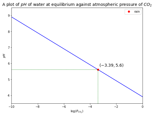
Given that \(P_{CO_2} = 409\,ppm = 10^{-3.39}\),
This indicates that water in equilibrium with atmospheric \(CO_2\) is acidic! If rain has a pH < 5.61, it is “acid” rain.
We can also find the activities of other species.
By (314), \(a_{HCO_{3}^{-}} = 10^{-5.61} \,mol/kg\)
By (315), \(a_{CO_{3}^{2-}} = 10^{-10.33} \,mol/kg\)
By (316), \(a_{OH^{-}} = 10^{-8.39} \,mol/kg\)
By eq5star, \(a_{H_2CO_3^{* }} = 10^{-4.86} \,mol/kg\)
Consider the equation below again:
Taking negative 10-base log, we get:
where \(c = \frac{pK_1 + pK_H}{2}\)
Then, we can plot the relationship between \(P_{CO_2}\) and \(pH\) of water at equilibrium with atmospheric \(CO_2\) as follows.
# function for calculating F_H, m_H2CO3, m_HCO3-, m_CO3--, m_H+, m_OH-
def pH_eq(pCO2):
    pK1 = 6.35
    pKH = 1.47
    c = (pK1+pKH)/2
    return -0.5*np.log10(pCO2) + c

# plot
plt.figure(figsize=(8,6))
pCO2 = np.linspace(10**-10, 1, 100)
log_pCO2_rain = -3.39
pH_rain = pH_eq(10**-3.39)
plt.plot(np.log10(pCO2), pH_eq(pCO2), 'b')
plt.plot(log_pCO2_rain, pH_rain, 'ro', label='rain')  # rain
plt.plot([log_pCO2_rain, log_pCO2_rain], [0, pH_rain], 'g:')
plt.plot([-10, log_pCO2_rain], [pH_rain, pH_rain], 'g:')
plt.text(-3.3, 5.8, r'$({0:.2f},{1:.1f})$'.format(log_pCO2_rain, pH_rain), fontsize=14)
plt.xlim([-10, 0])
plt.ylim([3.5, 9.5])
plt.xlabel('$\log(P_{CO_2})$')
plt.ylabel('$pH$')
plt.title('A plot of $pH$ of water at equilibrium against atmospheric pressure of $CO_2$', fontsize=14)
plt.legend(loc='best', fontsize=10)
<matplotlib.legend.Legend at 0x1fd60c6b850>
Lesson 4 - Problem 2#
a) Use the main relations linking the carbon system species to calculate the relative activity between \(H_2CO_3\) and \(HCO_3^-\) under the following conditions using the data in the table below:
\(\quad\)(i) At \(25^\circ C\) for a water sample whose \(pH=4.0\).
\(\quad\)(ii) At \(60^\circ C\) for a water sample whose \(pH=4.0\). How different is that from your previous answer in part i)?
# Table

# data
T = [0, 5, 10, 15, 20, 25, 30, 45, 60]
pK1 = [6.58, 6.52, 6.46, 6.42, 6.38, 6.35, 6.33, 6.29, 6.29]
pK2 = [10.63, 10.55, 10.49, 10.43, 10.38, 10.33, 10.29, 10.20, 10.14]

# create a dataframe
dict = {'T (C)' : T,
        'pK1' : pK1,
       'pK2' : pK2}
df = pd.DataFrame(dict)

# displaying the dataFrame
display(df.style.hide_index().set_precision(2))
| T (C) | pK1 | pK2 |
|---|---|---|
| 0 | 6.58 | 10.63 |
| 5 | 6.52 | 10.55 |
| 10 | 6.46 | 10.49 |
| 15 | 6.42 | 10.43 |
| 20 | 6.38 | 10.38 |
| 25 | 6.35 | 10.33 |
| 30 | 6.33 | 10.29 |
| 45 | 6.29 | 10.20 |
| 60 | 6.29 | 10.14 |
# create a function to calculate the relative activity between H2CO3 and HCO3- (a_H2CO3/a_HCO3-)
def H2CO3_HCO3_activity_ratio(pH, Temp):
    T = [0, 5, 10, 15, 20, 25, 30, 45, 60]
    pK1 = [6.58, 6.52, 6.46, 6.42, 6.38, 6.35, 6.33, 6.29, 6.29]
    if Temp in T:
        return 10**(-pH-(-pK1[T.index(Temp)]))
    else:
        return "No data for your input"

# (i)
T = 25; pH = 4
ratio_i = H2CO3_HCO3_activity_ratio(pH, T)
print(f"(i) There is {ratio_i:.0f} time more carbonic acid than bicarbonate ions in a water sample at \
{T} C and pH={pH}.")

# (ii)
T = 60; pH = 4
ratio_ii = H2CO3_HCO3_activity_ratio(pH, T)
print(f"(ii) There is {ratio_ii:.0f} time more carbonic acid than bicarbonate ions in a water sample at \
{T} C and pH={pH}.")

# compare
print(f"There is {ratio_ii:.0f}/{ratio_i:.0f}={ratio_ii/ratio_i:.2f} times as much bicarbonate at higher temperature.")
(i) There is 224 time more carbonic acid than bicarbonate ions in a water sample at 25 C and pH=4.
(ii) There is 195 time more carbonic acid than bicarbonate ions in a water sample at 60 C and pH=4.
There is 195/224=0.87 times as much bicarbonate at higher temperature.
b) Calculate the \(pH\) of rainwater at equilibrium with atmospheric \(CO_2\) at \(25^\circ C\) today? Assume that concentrations and activities are the same. The challenge of this question is to find a way to express \(pH\) (or \(a_{H^+}\)). This involves making simplifications to the charge balance equation: \(m_{H^+}=m_{HCO_3^-}+2m_{CO_3^{2-}}+m_{OH^-}\). The key being to argue that \(m_{H^+} \approx m_{HCO_3^-}\) for rain.
We have done that (\(pH=5.6\)).
c) A groundwater sample has a measured \(pH\) of \(6.84\) and a \(HCO_3^-\) concentration \(460\,mg/L\). Assuming that activity equal concentration, calculate the \(P_{CO_2}\) of this groundwater sample.
\(\quad\)(i) First, convert the units from \(mg/L\) to \(mol/kg\)
\(\quad\)(ii) Since we have \(pH\), we can use the expression between \(P_{CO_2}\) and \(HCO_3^-\):
and solve for \(P_{CO_2}\).
\(\quad\)(iii) How does the \(P_{CO_2}\) in that groundwater compare with the current atmospheric \(P_{CO_2}\) levels (\(409\,ppm\)). Will the \(CO_2\) contained in that sample remain in solution, or will it degas into the atmosphere?
(i)
(ii)
The expression of \(P_{CO_2}\) can be written as:
We can simplify by taking the log on both sides.
So, \(P_{CO_2} = 10^{-1.14} = 72443\,ppm\)!
(iii)
This is \(177\) times more than the current atmospheric \(P_{CO_2}\) levels, it is supersaturated. The \(CO_2\) contained in that sample will be released into the atmosphere is that water ever comes in contact with the atmosphere.
References#
Lecture slide and Practical for Lecture 4 of the Low-Temperature Geochemistry module