Divide and Conquer
Contents
Divide and Conquer#
Divide and Conquer algorithms are one of the major groups in computer problem-solving. The main idea is to split the more complicated tasks into independent subproblems that can be composed in the solution. The term is closely related to recursion, but the approach does not always lead to recursive solutions.
Examples#
Binary Search is a method of efficiently finding membership in a sorted list. Let us say we want to find if the element
xis inl:
Check the middle element of
lis equal tox, if yes, returnTrue, otherwise:
a) If the element is greater, search the right half of the array with the same procedure.
b) Otherwise, search the left half
Have a look at the iterative solution:
def binary_search(arr, x):
    low = 0
    high = len(arr) - 1
    mid = 0

    while low <= high:

        mid = (high + low) // 2

        # Check if x is present at mid
        if arr[mid] < x:
            low = mid + 1

        # If x is greater, ignore left half
        elif arr[mid] > x:
            high = mid - 1

        # If x is smaller, ignore right half
        else:
            return True

    # If we reach here, then the element was not present
    return False


l = [1,2,3,4,5]

print(binary_search(l,2))
print(binary_search(l,7))
True
False
This leads to the algorithm with \(O(\log(n))\) complexity. On each iteration, we decrease the size of the search space by a factor of 2.
Merge Sort Is a very famous and ingenious example of Divide and Conquer approach. The aim is to sort an array. This could be done using the Selection Sort which is \(O(n^2)\). Now, consider the following approach:
The list is of length 0 or 1: it is already sorted.
The list is longer: divide it into two lists of equal (almost equal) length and sort them using the general method. After those are returned, merge the two lists, so the resulting one is sorted.
Merging of the lists is executed by taking the minimum elements of the two lists and putting them in the resulting list until both lists are empty. This time we implement the algorithm recursively:
def merge(a, b):
    if len(a) == 0:
        return b
    elif len(b) == 0:
        return a
    res = []
    while len(a) > 0 and len(b) > 0:
        if a[0] <= b[0]:
            res.append(a.pop(0))
        else:
            res.append(b.pop(0))
    while len(a):
        res.append(a.pop(0))
    while len(b):
        res.append(b.pop(0))

    return res

def mergeSort(arr):
    if len(arr) < 2:
        return arr
    else:
        mid = len(arr)//2
        a = mergeSort(arr[:mid])
        b = mergeSort(arr[mid:])
        return merge(a,b)

print(mergeSort([3,2,1]))
print(mergeSort([2,3,2,2,4,7,8,9,3,6,7,3]))
print(mergeSort([]))
[1, 2, 3]
[2, 2, 2, 3, 3, 3, 4, 6, 7, 7, 8, 9]
[]
Now, let us consider the time complexity of this solution. On the merge of the two halves of the initial list we are performing roughly \(n\) operations. Then, merge of the halves was a result of \(2*n/2\) operations. The pattern is as follows:
So this algorithm is \(O(n\log(n))\). This is a considerable improvement compared to the Selection Sort.
Closest two points on a plane We are given a list of coordinates of points on a 2D Cartesian plane, find the minimum distance between any two points. The brute force solution is to check every pair of points in a list and find the minimum distance. This leads to \(O(n^2)\). However, there is a divide and conquer method which leads to a more efficient algorithm:
Base Case:
There are three points in a list - find their distance using brute force.
Recursive case:
Sort the points by the \(x\)-coordinate (can be done in \(O(nlog(n)\)).
Split the points into two groups (first and second half of the list).
Find the minimum distance of those two sublists by the same general procedure.
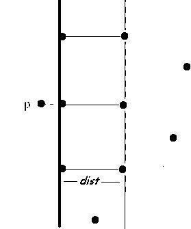
Let \(d_L\) and \(d_R\) denote the minimum distances from the left and right half. Now take the points that are at maximum \(min(d_L,d_R)\) from the middle point. This can be done in \(O(log(n))\) as the points are sorted. We build an array
stripfrom those points.Now sort the array
stripby the \(y\) coordinate.The tricky part: Intuition says that finding the minimum distance in the strip requires \(O(n^2)\) computation. However, let us notice the fact that each pair of points in one half is at minimum \(min(d_L,d_R)\) distance from each other. The only candidates for the new minimum distances are in the different halves. So we need to consider only the points in the
stripwhich have a difference of \(y\) coordinate that is less than \(min(d_L,d_R)\)! It can be proven geometrically that for each point, we need to check at most 6 other points. Therefore this operation is \(O(n)\). Please have a look at the following diagram for digesting this step.Find the minimum distance in the strip and return it.
Consider the code below:
from math import sqrt
import random

# for easier understanding of the code
class Point:
    def __init__(self,x,y):
        self.x = x
        self.y = y

# sqrt is uncessary computation, we will use it only in returning
# the final result
def dist(a,b):
    return (a.x-b.x)**2 + (a.y-b.y)**2


# This will be used for shorter lists
def bruteForce(P):
    assert len(P) > 1
    min_val = dist(P[0],P[1])

    for i in range(len(P)):
        for j in range(i+1, len(P)):
            if dist(P[i],P[j]) < min_val:
                min_val = dist(P[i],P[j])
    return min_val

def closestStrip(strip,d):
    # sort according to the y coordinate
    strip.sort(key = lambda point: point.y)
    min_val = d

    for i in range(len(strip)):
        j = i + 1
        # this loop is executed at most 6 times for each point
        while j < len(strip) and strip[j].y - strip[i].y < d:
            if dist(strip[j],strip[i]) < min_val:
                min_val = dist(strip[j],strip[i])
            j+=1

    return min_val

def helper(P):
    if len(P) <= 3:
        return bruteForce(P)
    mid = len(P) // 2
    d_L = helper(P[:mid])
    d_R = helper(P[mid:])
    d = min(d_L,d_R)
    #creating the strip
    strip = [a for a in P if abs(P[mid].x - a.x) < d]

    return min(d,closestStrip(strip,d))

def closestPoints(P):
    points = []
    for p in P:
        points.append(Point(p[0],p[1]))

    #sort according to the x coord.
    points.sort(key = lambda point: point.x)
    return sqrt(helper(points))


#testing the solution with bruteforce
for t in range(10):
    test = []
    for i in range(100):
        test.append(Point(random.randint(-100,100), random.randint(-100,100)))
    test.sort(key = lambda point: point.x)
    assert helper(test) == bruteForce(test)
Complexity analysis: Time complexity can be expressed as:
Where the \(O\) terms correspond to creating the stip list, sorting the strip by \(y\) coordinates and finding the minimum distance in the strip. This can be simplified by considering only the most contributing term.
This recurrence relation can be solved in various ways (e.g using the Master Theorem) and leads to \(O(n(log(n))^2)\).
Exercises#
Rotated Binary Search You are given a sorted list
arrwhich was rotated, which means that the elements were moved from indexito index(i+n)%len(arr)wherenis the amount of rotation. The example is:
[1,2,3,4,5,6] -> [5,6,1,2,3,4] is a rotation by 2.
Design an algorithm which finds the smallest element in \(O(log(n))\).
HINT: The elements on the sides of the smallest element are both greater than it.
Answer
# arr is sorted and rotated
def binaryRotated(arr, low, high):
    #base case
    if len(arr[low:high+1]) <= 3:
        min_val = arr[low]
        for i in arr[low:high+1]:
            if i < min_val:
                min_val = i
        return min_val

    mid = (low + high) // 2

    #minimum found
    if arr[mid-1] > arr[mid] and arr[mid+1] > arr[mid]:
        return arr[mid]
    #recursive cases
    elif arr[mid] > arr[0] and arr[mid] > arr[-1]:
        return binaryRotated(arr, mid,high)
    else:
        return binaryRotated(arr,low,mid-1)


# test the function
arr = [1,2,3,4,5,6,7,8,9,10]
for i in range(2*len(arr)):
    test = []
    for j in range(len(arr)):
        test.append(arr[(j+i) % len(arr)])
    #print(binaryRotated(test,0,len(arr)), test)
    assert min(arr) == binaryRotated(test,0,len(arr))
Quick Sort is probably the most widely used sorting algorithm in the world. In the worst case, it runs in \(O(n^2)\), but on average it is \(O(nlogn)\) with smaller constants than Merge Sort. The idea is as follows:
Base case:
List of length 1 is sorted, return
Recursive case:
Pick an element in the array (a pivot) and put the elements greater than the pivot in the left part of the array (or its copy for easier implementation) and greater elements in the right side of the array. Finally, insert the pivot in between. It is now in the place it should be in the sorted array.
Call
QuickSorton the subarray in the right of the pivot and on the subarray on the right of the pivot. The returned arrays will be sorted
Based on the above description, define a function QuickSort.
Answer
def QuickSort(arr):
    #base case
    if len(arr) == 1:
        return arr
    else:
        # setting the variables
        mid = len(arr) // 2
        pivot = arr[mid]
        left_border = 0
        right_border = len(arr) - 1
        copy = [0] * len(arr)

        #partitioning the array
        for i in range(len(arr)):
            if i != mid:
                if arr[i] <= pivot:
                    copy[left_border] = arr[i]
                    left_border += 1
                else:
                    copy[right_border] = arr[i]
                    right_border -= 1
        copy[left_border] = pivot

        #recursive calls
        if left_border > 0:
            copy[:left_border] = QuickSort(copy[:left_border])
        if right_border < len(arr) - 1:
            copy[right_border:] = QuickSort(copy[right_border:])
        return copy
References#
Sebastian Raschka, GitHub, Algorithms in IPython Notebooks
Cormen, Leiserson, Rivest, Stein, “Introduction to Algorithms”, Third Edition, MIT Press, 2009
GeeksforGeeks, Closest Pair of Points using Divide and Conquer algorithm