Pipe Flow with Heat

Geodynamics

(Lecture 7)

Following the 1D pipe flow problem in lecture 5, we now turn to problems involving both fluid flow and heat transfer.

Problem 6.26

Apply analysis to pressure-driven steady-state channel flow for no-slip walls. Assume \(dp/dx=1\), and \(y=-h/2\) to \(h/2\). We consider the case in which the wall temperature of the channel \(T_w\) is changing linearly along its length; that is,

(223)\[T_w (x) = C_1 x + C_2\]

where \(C_1\) and \(C_2\) are constants.

Accordingly, we consider the temperature of the fluid at any point (x,y) is given by

(224)\[T(x,y) = C_1 x +C_2 + \theta(y) = T_w(x) + \theta(y)\]

where \(\theta(y)\) is the difference between the fluid temperature and the wall temperature.

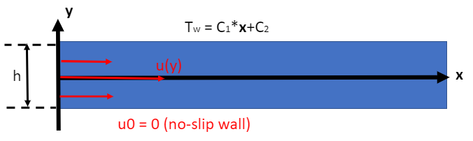
Figure 8.1

Derive the temperature equation in the cartesian coordinate.

First of all, let’s use the general equation for velocity we derived in lecture 5 for the same channel flow problem.

With the boundary conditions of \(u(y=\pm h/2)=0\), we have

(225)\[u(y) = \frac{1}{2\mu}\frac{dp}{dx}\left(y^2-\frac{h^2}{4}\right) = 3\bar{u}\left(\frac{1}{2}-\frac{2}{h^2}y^2\right)\]

(226)\[\bar{u}(y)=-\frac{1}{4\mu}\frac{dp}{dx}\frac{h^2}{3}\]

Then, we assume that the heat going into the system (i.e. any tiny red rectangle as shown in figure 8.2) equals to the heat going out of the system. This means that the net heat flowing into or out of the system due to wall heating should be the same amount of heat as the net heat flowing into or out of the system due to fluid flow. In a word, the net heat conduction in y-direction should be the same as the net heat advection in x-direction. However, we do not consider the heat being stored in the system, so the net heat rates must be balanced out.

The velocity profile we derived earlier will help us find the net heat advection in x-direction.

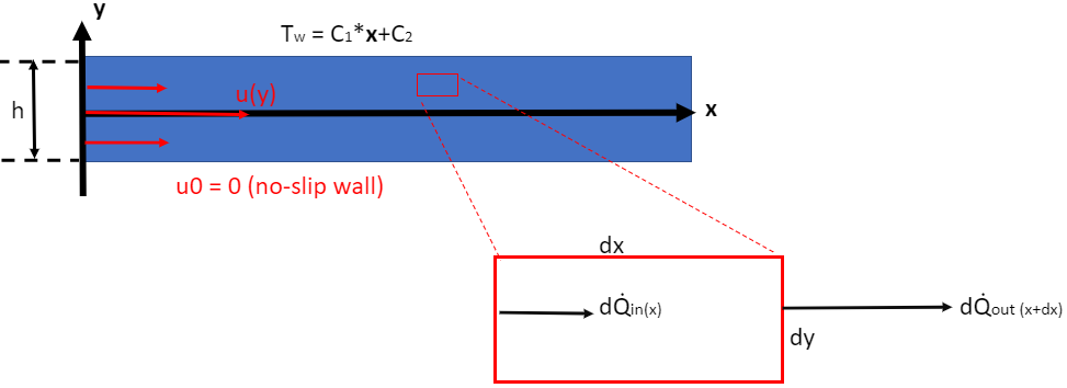
Figure 8.2

As shown in the figure 8.2, the net heat advection rate (in the tiny red rectangle) is

(227)\[\sum d\dot{Q}_{adv} = d\dot{Q}_{in} -d \dot{Q}_{out} = dy (u \rho c T(x) - u \rho c T(x+\delta x)) \]

Using the approximation that

(228)\[T(x+\delta x) = T(x)+\frac{\delta T}{\delta x}\cdot dx\]

We have the net rate of heat due to advection

(229)\[\sum d\dot{Q}_{adv} = -dy\cdot u\rho c \frac{\delta T}{\delta x}dx\]

We can write the equation (229) in another form by replacing velocity \(u\) with \(\frac{dx}{dt}\) to understand the physical unit (since we are all familiar with the famous equation \(Q=cm\Delta T\)).

(230)\[\sum d\dot{Q}_{adv} = -dy \frac{dx}{dt}\rho c \frac{dT}{dx}dx = \frac{c \cdot dm \cdot \Delta T}{t}\]

where tiny mass of red rectangle \(dm = dx dy \rho\)

Since we know that the derivative of temperature \(T(x,y)\) in (229) wrt. \(x\) is \(C_1\), and the velocity \(u(y)\) from (225), we can rewrite (229) as

(231)\[\sum d\dot{Q}_{adv} = -dy \cdot 3\bar{u}\left(\frac{1}{2}-\frac{2}{h^2}y^2\right) \cdot \rho c \cdot C_1dx\]

Next, we study the net heat conduction rate in the y-direction due to wall heating.

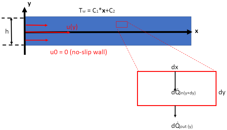
Figure 8.3: Thickness of the channel \(h\) is also represented by \(d\) since \(h\) is used as heat transfer coefficient later.

(232)\[\sum d\dot{Q}_{con} = d\dot{Q}_{in} -d \dot{Q}_{out} = dx (q_x(y+\delta y) - q_x(y)) \]

where heat flux \(q_x = - k \frac{\delta T}{\delta y}\), and \(k\) is the thermal conductivity of the fluid.

Again, using the first term of the Taylor expansion to approximate \(q_x(y+\delta y)\), we have

(233)\[q_x(y+\delta y) = q_x(y)+\frac{dq_x}{dy}\cdot dy\]

So equation (232) becomes

(234)\[\sum d\dot{Q}_{con} = dx \frac{dq_x}{dy}dy = - dx \cdot k \frac{\delta^2 T}{\delta y^2}dy\]

Finally, as we said before, the net heat rate of the system should be balanced by the conduction and convection. So we combine (231) and (234), and have

(235)\[\sum d\dot{Q}_{con} + d\dot{Q}_{adv} = - dx \cdot k \frac{\delta^2 T}{\delta y^2}dy -dy \cdot 3\bar{u}\left(\frac{1}{2}-\frac{2}{h^2}y^2\right) \cdot \rho c \cdot C_1dx = 0 \]

where \(\frac{\delta^2 T}{\delta y^2}=\frac{\delta^2 \theta}{\delta y^2}\) from (224).

Rearrange (235), we have an equation of \(\frac{\delta^2 \theta}{\delta y^2}\)

(236)\[\frac{\delta^2 \theta}{\delta y^2} = \frac{6 \bar{u}}{k h^2}\rho c C_1 y^2 - \frac{3\bar{u}}{2k}\rho c C_1\]

Integrate it twice, and apply two boundary conditions (\(\frac{\delta \theta}{\delta y}=0\) at \(y=0\) and \(\theta = 0\) at \(y = \pm h/2\)), we will arrive at

(237)\[\theta(y)=\frac{ \rho cC_1}{4k\mu}\frac{dp}{dx}\left(\frac{1}{6}y^4-\frac{1}{4}h^2y^2+\frac{5}{96}h^4\right)\]

Using \(\frac{1}{\kappa} = \frac{\rho c}{\mu}\), \(\frac{dp}{dx}=1\) and \(d=h\) to rewrite equation (237), we will have the same answer as the book

(238)\[\theta(y)=\frac{ C_1}{4\kappa\mu}\left(\frac{1}{6}y^4-\frac{1}{4}d^2y^2+\frac{5}{96}d^4\right)\]

Finally, we have

(239)\[T(x,y) = T_w(x) + \theta(y) = C_1x + C_2 + \frac{ C_1}{4\kappa\mu}\left(\frac{1}{6}y^4-\frac{1}{4}d^2y^2+\frac{5}{96}d^4\right)\]

from mpl_toolkits import mplot3d
import numpy as np
import matplotlib.pyplot as plt
N  = 100    # number of points to plot (ignore)
mu = 0.001    # viscosity of water
dpdx = 1    # when pressure difference = 0, known as Couette flow
h = 0.1    # thickness of channel (m)
d = h    # we use d to denote thickness h because h is later used to represent heat transfer coefficient
C1 = 0.01    # temperature rise 1 degree every 1000 m
C2 = 10
rho = 1000    # density of water
c = 4190    # specific heat capacity of water
k = 4    # thermal conductivity of water at 20 degree = 4.18 in SI unit
kappa = k/(rho*c)    # thermal diffusivity, sometimes called alpha
x_range = 200    # length of the channel


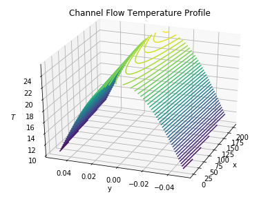
def T(x, y):
    return C1*x +C2 + C1/(4*kappa*mu)*( (1/6)*y**4 - ((1/4)*d**2) * y**2 + (5/96)*d**4 )


x = np.linspace(0, x_range, N)
y = np.linspace(-d/2, d/2, N)

X, Y = np.meshgrid(x, y)
Z = T(X, Y)

fig = plt.figure(figsize=(7, 5))
ax = plt.axes(projection='3d')
ax.contour3D(X, Y, Z, 50)
ax.set_xlabel('x')
ax.set_ylabel('y')
ax.set_zlabel('$T$')
ax.view_init(30, 200)
ax.set_title('Channel Flow Temperature Profile')
plt.show()

Then, we can work out the wall heat flux (\(q_x\) at \(y=d/2\))

(240)\[q_{x}=-k\frac{\delta T}{\delta y}=\frac{C_1 k d^3}{24\kappa \mu}\]

The heat flux is thus a constant, independent of \(y\). If \(C_1\) is positive, the wall temperature increases in the direction of flow, and heat flows through the wall of the pipe into the fluid. If \(C_1\) is negative, the wall temperature decreases in the direction of flow, and heat flows out of the fluid into the wall of the pipe. The heat flux to the wall can be expressed in a convenient way by introducing a heat transfer coefficient \(h\) between the wall heat flux and the excess fluid temperature according to

(241)\[q_{x}=h(\bar{T}-T_w)=h\bar{\theta}\]

where the overbar represents an average over the cross section of the channel.

The average is weighted by the flow per unit area, that is, the velocity through \(dy\) in 2D. Thus the flow-weighted average excess fluid temperature is

(242)\[\bar{\theta}=\frac{1}{d\bar{u}}\int^{d/2}_{-d/2}\theta u \,dy\]

where the result can be obtained from WolframAlpha.

(243)\[h=\frac{q_x}{\bar{\theta}}=\frac{70k}{17d}\]

Note that the (243) is valid only for Reynolds numbers less than about 2200. At higher values of the Reynolds number the flow is turbulent.

The fluid mechanics literature commonly introduces a dimensionless measure of the heat transfer coefficient known as the Nusselt number \(Nu\). For pipe flow with heat addition,

(244)\[Nu=\frac{hd}{k}=\frac{\frac{70k}{d}d}{k}\]

The Nusselt number measures the efficiency of the heat transfer process. If the temperature difference \(\bar{T} −T_w\) were established across a stationary layer of fluid of thickness \(D\) and thermal conductivity \(k\), the conductive heat flux \(q_c\) would be

(245)\[q_{c}=\frac{k(\bar{T}-T_w)}{d}\]

Thus the Nusselt number can be written as the ratio of convective to conductive heat transfer at a boundary in a fluid.

(246)\[Nu=\frac{q_x}{q_c}\]

Problem 6.28

The results of this section were based on the assumption of a laminar heat transfer coefficient for the aquifer flow. Because this requires \(Re < 2200\), what limitation is placed on the Peclet number?

The Peclet number is a dimensionless measure of the mean velocity of the flow through the aquifer. It is related to the dimensionless parameters \(Re\) and \(Pr\) already introduced. Since the thermal diffusivity \(\kappa\) is \(k/\rho c\), \(Pe\) can be written as

(247)\[Pe=\frac{\rho c \bar{u}R}{k}=\frac{\bar{u}R}{\kappa}\]

If the flow is turbulent, then the mean velocity of the fluid is likely to be reduced because some streams would be flowing in the opposite direction as the other streams. Therefore, the \(Pe\) number would be low in reality but high in calculations.