Introduction to waves

Waves

In this notebook, wave properties will be discussed, as well as derivations for simple harmonic motion and the wave equation.

import numpy as np
import matplotlib.pyplot as plt

Wave properties

A summary of the wave properties can be seen in the figure below:

Selection of wave properties:

• \(t\) – time

• \(A\) – amplitude

• \(f\) – frequency, \(f = \frac{\omega}{2\pi}\)

• \(\lambda\) – wavelength, \(\lambda = vf = \frac{2\pi}{k}\)

• \(T\) – period, \( T = \frac{1}{f}\)

• \(p\) – phase shift

• \(\omega\) – angular frequency

• \(k\) – wave number

• \(c_p\) – phase speed, \(c_p = \frac{\omega}{k}\)

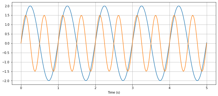
A variation and comparison between a selection of wave properties can be seen below:

def sine_wave(t, A, f, p):
    """
    This formula will be derived later on for simple harmonic motion using Newton's 2nd law
"""
    y = A*np.sin(2*np.pi*f*t + p*np.pi/180)
    return y

t = np.linspace(0,5,200)

A1 = 2
f1 = 1
p1 = 1
y1 = sine_wave(t, A1, f1, p1)

A2 = 1.5
f2 = 2
p2 = 0.2
y2 = sine_wave(t, A2, f2, p2)

plt.figure(figsize=(12,5))
plt.xlabel("Time (s)")
plt.plot(t, y1)
plt.plot(t, y2)
plt.grid(True)
plt.show()

Simple Harmonic Motion

A wave carries information and energy but does not transport the material. It undergoes simple harmonic motion.

To derive the formula for simple harmonic motion (SHM), assume an object of mass m and mean position \(y_0\) and the displacement ‘\(y\)’. In SHM, there is a restoring force that is directed towards the mean position \(y_0\) at every instant. The restoring force is directly proportional to the displacement of the body at every instant, so \(F \propto -y\). The negative sign indicates that the restoring force acts opposite to the displacement. Thus, including the force constant, \(k\),

\[F = -ky \qquad (1)\]

Now consider Newton’s second law of motion \(F = ma\), where \(F\) is the restoring force on the body, \(m\) is the mass and \(a\) is the acceleration.

Since \(a = \frac{dv}{dt}= \frac{d^2 y}{d t^2}\), so

\[F = m \frac{d^2 y}{d t^2} \qquad (2)\]

Combining equations (1) and (2), we get

\[m \frac{d^2 y}{d t^2} = -ky\]

\[\frac{d^2 y}{d t^2} = - \frac{k}{m}y\]

\[\frac{d^2 y}{d t^2} + \frac{k}{m}y = 0\]

Let \(\frac{k}{m} = \omega^2\). Now,

\[\frac{d^2 y}{d t^2} + \omega^2 y = 0 \qquad (3)\]

The solution to this equation can be approximated from analysis, knowing that a sin or cosine function when differentiated twice returns to it’s original form, with a factor in front. So, we can estimate the solution to be

\[ y = A \sin(\omega t)\]

As we know that

\[v = \frac{dy}{dt} = A\omega \sin(\omega t)\]

and

\[a = \frac{d^2y}{dt^2} = A\omega^2 \sin(\omega t)\]

Filling \( y = A \sin(\omega t)\) back into equation (3), we get

\[ A\omega^2 \sin(\omega t) + A \sin(\omega t) \cdot \omega^2\]

which shows that this solution is valid.

Thus, the solution to the wave equation is:

\[ y = A \sin(\omega t) = A \sin (2 \pi f t)\]

Here, \(A\) is the magnitude of the initial displacement, \(\omega\) is the angular frequency and \(t\) is time.

def displacement(t, A, f):
    y = A*np.sin(2*np.pi*f*t)
    return y

def velocity(t, A, f):
    v = A*2*np.pi*f*np.cos(2*np.pi*f*t)
    return v

def acceleration(t, A, f):
    a = A*(2*np.pi*f)**2*np.sin(2*np.pi*f*t)
    return a

t = np.linspace(0,5,200)

A = 2
f = 1
displacement = displacement(t, A, f)
velocity = velocity(t, A, f)
acceleration = acceleration(t, A, f)

plt.figure(figsize=(12,5))
plt.xlabel("Time (s)")
plt.plot(t, displacement, label = "displacement (m)")
plt.plot(t, velocity, label = "velocity (m/s)")
plt.plot(t, acceleration, label = "acceleration ($m^2$/s)")
plt.grid(True)
plt.legend()
plt.title("Relationship of displacement, velocity and acceleration")
plt.show()

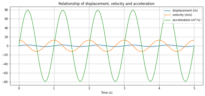
Note a few things in the plot above:

• Velocity is zero where particle displacement is at it’s maximum or minimum.

• Velocity is at it’s maximum or minimum when the particle displacement goes through the equilibrium position.

• When particle displacement is at the equilibrium position, acceleration is zero.

• Acceleration has a maximum or minimum when the particle displacement has a maximum or minimum.

Using trigonometry,

\[F = ma = -mg\sin(\theta)\]

Thus,

\[a = g\sin(\theta)\]

Approximate that for small \(\sin(\theta) = \theta\), so

\[F = ma = mg\theta = m \frac{y}{l}\]

Thus,

(317)\[a = \frac{F}{ml}y \text{.}\]

If the restoring force is tension from a string for example, it can be approximated as \(F=-2T\), considering a string pulls the body from the left and right side.

The equation of simple harmonic motion then becomes:

\[\frac{d^2 y}{d t^2} = - \frac{2T}{ml} y = -\omega ^2 y \]

Wave equation

To derive the wave equation, a string with density \(\rho\) per unit length is stretched in the \(x\) direction with tension force \(T\). A wave can be described as coupled simple harmonic motion. This can be thought of as a rope with lots of masses being displaced individually.

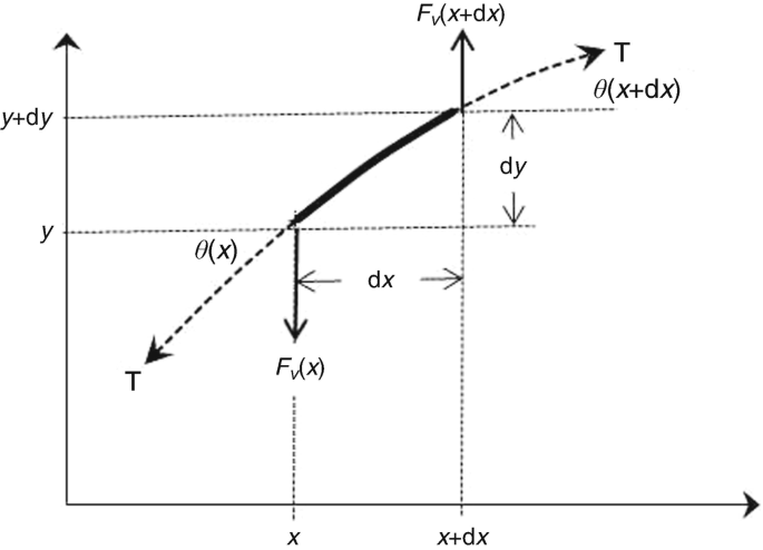
The vertical forces on the string must balance.

Consider Newton’s second law for the force, where \(F=ma\)

Consider \(m=\rho\Delta x\), as \(m = \rho V\) and only one dimension is considered. So, force is

\[ma=\rho \Delta x \cdot \frac{\partial ^2 u}{\partial t^2}\]

This is equal to the difference between the vertical tension T at the two ends, so

\[\rho \Delta x \cdot \frac{\partial ^2 u}{\partial t^2} = T(x+ \Delta x, t)\sin\left[\theta(x+\Delta x, t)\right] - T(x,t)\sin\left[\theta(x,t)\right]\]

Assume that the deflection angles \(\theta\) are small, \(\sin\theta = \tan\theta = \frac{\partial u}{\partial x}\). Thus,

\[\rho \Delta x \cdot \frac{\partial ^2 u}{\partial t^2} = T(x+ \Delta x, t)\frac{\partial u}{\partial x} - T(x,t)\frac{\partial u}{\partial x}\]

Divide both sides by \(\Delta x\) and letting \(\Delta x \rightarrow 0\) gives:

\[\rho(x)\frac{\partial^2 u}{\partial t^2} = \frac{\partial}{\partial x}\left(T \frac{\partial u}{\partial x}\right)\]

Assuming deflection is small, \(T\) can be assumed to be constant.

Considering \(c^2 = \frac{T}{\rho}\), the wave equation becomes

\[\frac{\partial^2 u}{\partial t^2} = c^2 \frac{\partial^2 u}{\partial x^2}\]

One solution to the wave equation is by using travelling waves of the form \(u(x,t) = f(x \pm ct)\).

At \(t=0\), \(f(x)\) is a shape in space.

\(f(x-ct)\) is the shape of \(f(x)\) when travelling to the right at speed \(c\).

\(f(x+ct)\) is the shape of \(f(x)\) when travelling to the left at speed \(c\).

To plot the wave equation, a few initial conditions have to be set. consider

Types of waves

Body waves

• Longitudinal waves: waves where the displacement of the medium is in the same direction as the travelling wave. Examples are P-waves or sound waves.

• Transverse wave: waves where motion of all points oscillate in a path that is perpendicular to the direction of the travelling wave. Examples are seismic S-waves, electro-magnetic waves and vibrations on string.

Surface waves

• Love wave: wave moving horizontally and perpendicular to the direction of travel.

• Rayleigh wave: wave causing elliptical retrograde motion (opposite to direction of travel) in the vertical plane along direction of travel as a combination of both longitudinal and transverse vibration.

• Water wave: circular motion of elements moving in the same direction of wave travel.

References

Imperial College waves lecture notes