First-order linear PDEs

Mathematics for Scientists and Engineers 2

In this section we will consider first-order linear PDEs for an unknown function \(u\) of two variables:

\[ a(x,y)u_x + b(x,y)u_y = f(x, y, u) \]

The method which we will use to find the solution of such PDEs is called the method of characteristics. This is a very useful method with an intuitive geometric interpretation and it can be applied to even more complicated PDEs, which we will not consider here.

Method of characteristics

The main idea behind this method is a popular one: we want to reduce the PDE to an ODE, which are in general much easier to solve. We do that by analysing the PDE along specially chosen curves in \(xy\) plane, which we call characteristic curves or just characteristics. We parameterise them by the parameter \(s\), such that \(x = x(s), y = y(s)\) and we choose them such that the following system of ODEs is satisfied:

\[ \frac{dx}{ds} = a, \quad \frac{dy}{ds} = b, \quad \frac{du}{ds} = f\]

Then after using the chain rule and substituting this, we have

\[ \frac{du}{ds} = \frac{\partial u}{\partial x} \frac{dx}{ds} + \frac{\partial u}{\partial y} \frac{dy}{ds} = f(x(s), y(s), u(s)) \]

This simplifies our problem quite a bit, since we have reduced the PDE to an ODE. Let us now look at a few examples.

Example: constant coefficients, homogeneous

Let us start with the simplest example, where \(a\) and \(b\) are constants and \(f \equiv 0\):

\[ 2u_x + 3u_y = 0, \qquad u(x, 0) = \cos x \]

Setting

\[ \frac{dx}{ds} = 2, \quad \frac{dy}{ds} = 3\]

and using the chain rule we get

\[ \frac{du}{ds} = 2u_x + 3u_y = 0 \]

This means that the PDE along the characteristic line \((x(s), y(s))\) is a constant. We can write the parametrization invariant form of the above equations as

\[ ds = \frac{dx}{2} = \frac{dy}{3} \]

from which

\[ \frac{dx}{dy} = \frac{2}{3} \]

So the characteristics are given by \(2y = 3x + c\), where \(c\) is an integration constant which will determine which characteristic line we are on. Let us plot a couple of them.

import numpy as np
import matplotlib.pyplot as plt


x = np.linspace(-5, 5, 51)
c = np.linspace(-10, 10, 9)

fig, ax = plt.subplots(1, 1, figsize=(6, 6))

for cc in c:
    ax.plot(x, 3/2 * x + cc, 'k-', alpha=0.3)
    
    if cc > -5:
        ax.text(2 - cc/1.5, 3, cc, c='darkblue', weight='bold')

ax.text(-0.1, 5.4, 'y', weight='bold')
ax.text(5.7, -0.1, 'x', weight='bold')
        
ax.set_aspect('equal')
ax.spines['left'].set_position('zero')
ax.spines['bottom'].set_position('zero')
ax.spines['right'].set_visible(False)
ax.spines['top'].set_visible(False)
ax.set_ylim(-5, 5)
    
plt.show()

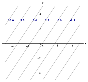
Here we plotted characteristics for different values of \(c\), which are written in bold along characteristics.

All characteristics are parallel to each other, of course, and since \(u\) is constant along each characteristic line, \(u\) will only vary if we jump from one characteristic to another. Since \(c\) marks which characteristic we are sitting on, \(u\) will therefore be a function of \(c\).

\[ u(x(y), y) = f(c) = f(-3x + 2y) \]

where \(f\) is an arbitrary function of one variable.

Finally we need to use the auxiliary condition \(u(x, 0) = \cos x\) to find the particular solution. For \(y=0\):

\[ u(x, 0) = f(-3x) = \cos (x) \]

Let \(w = -3x\). Then,

\[ f(w) = \cos (-w/3) \text{.}\]

Hence the solution is

\[ u(x, t) = f(-3x + 2y) = \cos(x - \frac{2}{3}y) \]

from mpl_toolkits.mplot3d import Axes3D


x = np.linspace(-5, 5, 201)
y = np.linspace(-5, 5, 201)
X, Y = np.meshgrid(x, y)

f = np.cos(X - 2/3 * Y)

fig = plt.figure(figsize=(10, 8))

ax1 = fig.add_subplot(121, projection='3d')
ax2 = fig.add_subplot(122)

ax1.plot_surface(X, Y, f, rstride=1, cstride=1, cmap='inferno', antialiased=False)
ax2.contourf(f, cmap='inferno', extent=[-5, 5, -5, 5])
ax2.contour(f, colors='k', extent=[-5, 5, -5, 5], linewidths=1.)

ax1.view_init(40, 70)
ax2.set_aspect('equal')

for ax in (ax1, ax2):
    ax.set_xlabel('x')
    ax.set_ylabel('y')
ax1.set_zlabel('u')
    
fig.suptitle(r'$u(x,y) = \cos (x - \frac{2}{3}y)$')

plt.tight_layout()
plt.show()

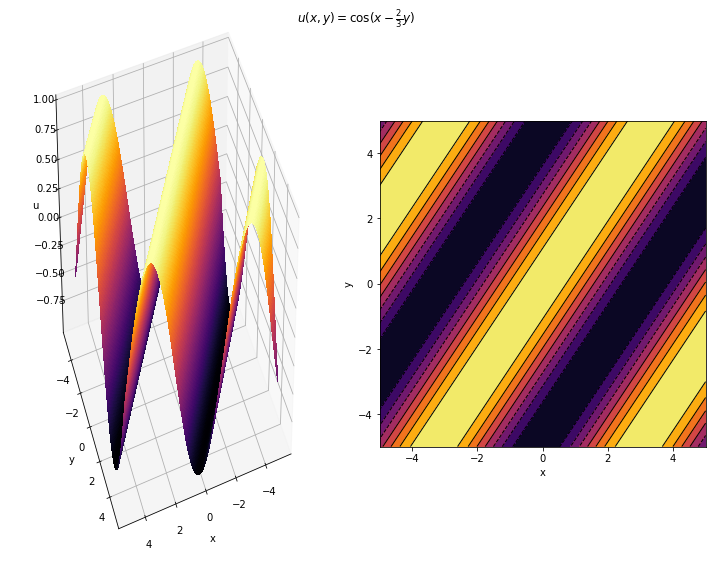
Notice that each of the contours is a characteristic, since \(u\) is constant along a characteristic.

Important

A first-order linear PDE of the form

\[ au_x + bu_y = 0 \]

has a general solution of the form

\[ u(x, y) = f(bx - ay) \]

where \(f\) is an arbitrary function of one variable.

Example: general case

Let us now consider an inhomogeneous linear problem with variable coefficients.

\[ (x + y)u_x + y u_y = xyu \]

with the boundary condition \(u(x,y) = e^{x^2/4} \) for \(y = x\).