Elementary functions 1

Mathematics for Geoscientists

In this notebook we define some of the most common functions in general mathematics. Readers might be familiar with most of this content from school, but it will serve as a nice transition point towards more rigorous sections. This notebook should also serve as a small collection of examples for previous notebooks in this section.

Polynomial function

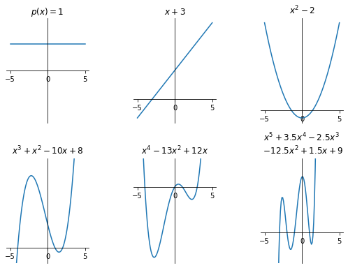
A polynomial of degree \(n \in \mathbb{N}\) is a real function of a real variable given by the formula:

\[ p_n(x) = a_n x^n + a_{n-1} x^{n-1} + \dots + a_1x + a_0, \]

where \(a_0, a_1, \dots, a_n \in \mathbb{R}\) are the polynomial coefficients such that \(a_n \neq 0\). The natural domain of polynomial functions is the entire \(\mathbb{R}\).

import numpy as np
import matplotlib.pyplot as plt


x = np.linspace(-5, 5, 100)
titles = [['$p(x)=1$', '$x + 3$' ,'$x^2 - 2$'], 
          ['$x^3 + x^2 - 10x + 8$', '$x^4 - 13x^2 + 12x$' ,'$x^5 + 3.5x^4 - 2.5x^3$ \n $- 12.5x^2 + 1.5x + 9$']]

fig, ax = plt.subplots(2, 3, figsize=(8, 6))
fig.tight_layout(pad=3.)

ax[0, 0].plot(x, [1] * len(x))
ax[0, 1].plot(x, x + 3)
ax[0, 2].plot(x, x**2 - 2)
ax[1, 0].plot(x, x**3 + x**2 - 10*x + 8)
ax[1, 1].plot(x, x**4 - 13*x**2 + 12*x)
ax[1, 2].plot(x, x**5 + 3.5*x**4 - 2.5*x**3 - 12.5*x**2 + 1.5*x + 9)

ax[0, 0].set_ylim(-2, 2)
ax[1, 0].set_ylim(-5, 30)
ax[1, 1].set_ylim(-80, 30)
ax[1, 2].set_ylim(-5, 12)

for i in range(2):
    for j in range(3):
        ax[i, j].spines['left'].set_position('zero')
        ax[i, j].spines['bottom'].set_position('zero')
        ax[i, j].spines['right'].set_visible(False)
        ax[i, j].spines['top'].set_visible(False)
        ax[i, j].set_title(titles[i][j])
        ax[i, j].set_yticks([])

plt.show()

Linear functions

Quadratic functions

A function given by the formula \( f(x) = ax^2 + bx + c, a \neq 0 \) is called the quadratic function. We call its graph a parabola. The roots of a quadratic function are given by:

The quadratic function can be written in vertex form as \(f(x) = a \left ( x + \frac{b}{2a} \right ) + c - \frac{b^2}{4a}\) from which we see that its vertex position is

\[ \left ( - \frac{b}{2a}, - \frac{D}{4a} \right ), \]

where the number

\[D := b^2 - 4ac\]

is called the discriminant of a quadratic function. The discriminant is important because it tells us about the null-points (roots) of the function, which are given by

\[ x_{1,2} = \frac{-b \pm \sqrt{b^2 - 4ac}}{2a} = \frac{-b \pm \sqrt{D}}{2a}. \]

Therefore, if:

• \(D < 0\), no real roots, i.e. \(x_1, x_2 \notin \mathbb{R}\)

• \(D = 0\), one real root i.e. \(x_1, x_2 \in \mathbb{R} : x_1 = x_2\)

• \(D > 0\), two real roots, i.e. \(x_1, x_2 \in \mathbb{R} : x_1 \neq x_2\)

Rational functions

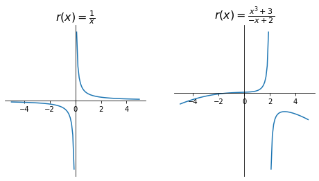
A rational function is a real function of a real variable given by the formula:

\[ r(x) = \frac{p(x)}{q(x)}, \]

where \(p\) and \(q\) are real polynomials. The natural domain of \(r(x)\) is the entire \(\mathbb{R}\) without the null-points of \(q(x)\) (we cannot divide by zero). That is, \(r(x)\) is defined on \(\mathbb{R} \backslash \{ x \in \mathbb{R} : q(x) = 0 \}\).

# for demonstration purposes will suppress warnings when div by 0
import warnings; warnings.simplefilter('ignore')


x = np.linspace(-5, 5, 101)

fig, ax = plt.subplots(1, 2, figsize=(8, 4))

ax[0].plot(x, 1/x)
ax[0].set_title(r'$r(x) = \frac{1}{x}$', fontsize=16)

ax[1].plot(x, (x**3 + 3)/(-x + 2))
ax[1].set_title(r'$r(x) = \frac{x^3 + 3}{-x + 2}$', fontsize=16)

for i in range(2):
    ax[i].spines['left'].set_position('zero')
    ax[i].spines['bottom'].set_position('zero')
    ax[i].spines['right'].set_visible(False)
    ax[i].spines['top'].set_visible(False)
    ax[i].set_yticks([])

plt.show()

Exponential function

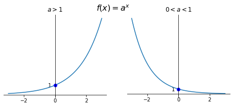
An exponential function is a function of the form

\[ f(x) = a^x, \qquad a \in \mathbb{R}^+ \backslash \{ 1 \}, \]

where \(a\) is called the base and is a positive real number different from \(1\). A special case of an exponential function is the natural exponential function \(f(x) = e^x\) where the base is \(e \approx 2.718282...\) (Euler’s number).

The natural domain of an exponential function is the entire set \(\mathbb{R}\) and its image is \((0, + \infty)\), i.e. \(a^x > 0, \forall x \in \mathbb{R}\). Exponential function \(x \mapsto a^x\) always crosses the y-axis at point \((0, 1)\) since \(a^0 = 1\).

Exponential function \(f(x) = a^x\) is:

• strictly increasing if \(a > 1\)

• strictly decreasing if \(0 < a < 1\)

x = np.linspace(-3, 3, 100)

fig, ax = plt.subplots(1, 2, figsize=(8, 3))
fig.suptitle(r'$f(x) = a^x$', fontsize=16)

ax[0].plot(x, 2**x)
ax[0].set_title(r'$a > 1$')

ax[1].plot(x, 0.4**x)
ax[1].set_title(r'$0 < a < 1$')

for i in range(2):
    ax[i].plot(0, 1, 'bo')
    ax[i].spines['left'].set_position('zero')
    ax[i].spines['bottom'].set_position('zero')
    ax[i].spines['right'].set_visible(False)
    ax[i].spines['top'].set_visible(False)
    ax[i].set_yticks([1])

plt.show()

Hyperbolic functions

Using the exponential function we define hyperbolic functions as follows:

\[\begin{split} \begin{aligned} \sinh x & := \frac{e^x - e^{-x}}{2} \\ \cosh x & := \frac{e^x + e^{-x}}{2} \\ \tanh x & := \frac{\sinh x}{\cosh x} = \frac{e^{2x} - 1}{e^{2x} + 1} \\ \coth x & := \frac{\cosh x}{\sinh x} = \frac{e^{2x} + 1}{e^{2x} - 1} \end{aligned}\end{split}\]

x = np.linspace(-2.5, 2.5, 100)

fig, ax = plt.subplots(1, 2, figsize=(10, 5))

ax[0].plot(x, np.sinh(x), label=r'$sinh(x)$')
ax[0].plot(x, np.cosh(x), label=r'$cosh(x)$')

ax[0].plot(x, np.exp(-x) / 2, '--k', alpha=0.3)
ax[0].plot(x, np.exp(x)/2, '--k', alpha=0.3)
ax[0].text(-2, 0.4, r'$\frac{1}{2}e^x$')
ax[0].text(2, 0.4, r'$\frac{1}{2}e^{-x}$')

ax[1].plot(x, np.tanh(x), label=r'$tanh(x)$')
ax[1].plot(x, 1 / np.tanh(x), label=r'$coth(x)$')

ax[1].set_ylim(-2, 2)
ax[1].hlines(1, -2.5, 2.5, linestyles='--', alpha=0.3)
ax[1].hlines(-1, -2.5, 2.5, linestyles='--', alpha=0.3)
ax[1].set_yticks([-2, -1, 1, 2])

for i in range(2):
    ax[i].spines['left'].set_position('zero')
    ax[i].spines['bottom'].set_position('zero')
    ax[i].spines['right'].set_visible(False)
    ax[i].spines['top'].set_visible(False)
    ax[i].legend(loc='best')
    
plt.show()

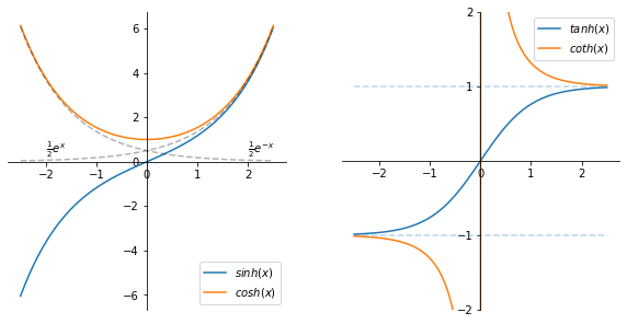
Properties

	\(\sinh x\)	\(\cosh x\)	\(\tanh x\)	\(\coth x\)
Domain	\(\mathbb{R}\)	\(\mathbb{R}\)	\(\mathbb{R}\)	\(\mathbb{R} \backslash \{ 0 \}\)
Image	\(\mathbb{R}\)	\((1, + \infty)\)	\((-1, 1)\)	\((- \infty, -1) \cup (1, + \infty)\)
Monotonic?	strictly increasing	strictly decreasing on \((- \infty, 0]\), strictly increasing on \([0, + \infty)\)	strictly increasing	strictly decreasing on \((- \infty, 0)\) and \((0, + \infty)\)
Even/odd?	Odd	Even	Odd	Odd

Similar to the Pythagorean trigonometric identity, the principal formula for hyperbolic functions is:

\[ \cosh^2 x - \sinh^2 x = 1. \]

Also similar are the argument addition and subtraction formulae:

\[ \sinh (x \pm y) = \sinh x \cosh y \pm \cosh x \sinh y \]

\[ \cosh (x \pm y) = \cosh x \cosh y \pm \sinh x \sinh y \]

Trigonometric functions

The radian is a measurement of the angle formed by two radii of a unit circle connecting the circle arc of unit length. \(2 \pi rad = 360^\circ\)

A function \(f: \mathcal{D} \to \mathbb{R}\) is periodic with a period \(\tau > 0\) if for all \(x \in \mathcal{D}\):

1. \( x + \tau \in \mathcal{D} \)

2. \(f(x + \tau) = f(x)\).

Note that if \(\tau\) is a period of a function, any multiple of it is also a period of the same function. We therefore define the fundamental period (also primitive, basic and prime period) as the smallest positive period.

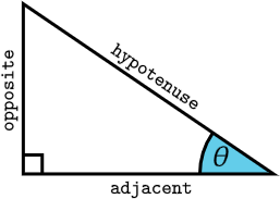The six trigonometric functions are sine, cosine, tangent and their inverses cosecant, secant, cotangent, respectively. We can define them for acute angle \(\theta\) in right-angled triangles as follows:

\[ \sin \theta = \frac{\text{opposite}}{\text{hypotenuse}}, \quad \cos \theta = \frac{\text{adjacent}}{\text{hypotenuse}}, \quad \tan \theta = \frac{\text{opposite}}{\text{adjacent}}\]

And their inverses:

\[\csc \theta = \frac{\text{hypotenuse}}{\text{opposite}}, \quad \sec \theta = \frac{\text{hypotenuse}}{\text{adjacent}}, \quad \cot \theta = \frac{\text{adjacent}}{\text{opposite}}\]

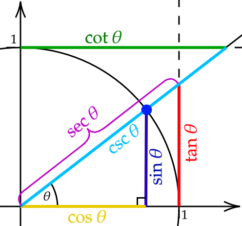
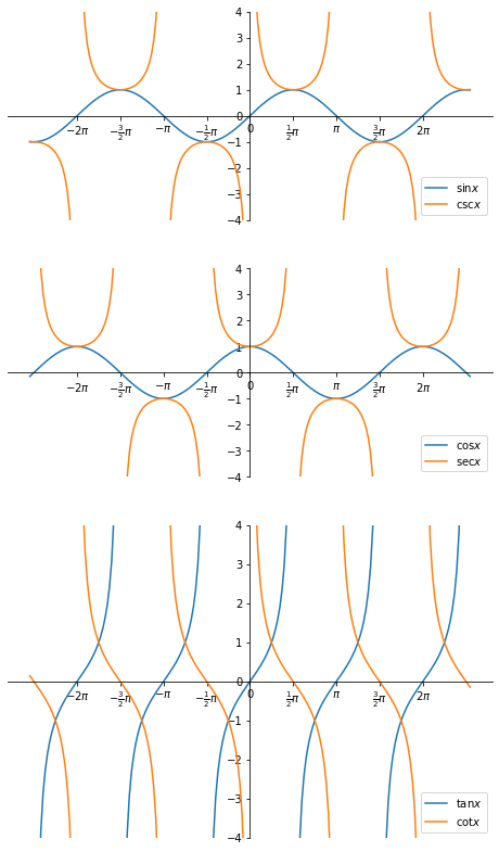
To extend the definitions of trigonometric functions to the entire set \(\mathbb{R}\) we could consider a unit circle centered at the origin. The \(x\) and \(y\) coordinates of a point on a circle is then \(\cos \theta\) and \(\sin \theta\), respectively, where \(\theta\) is the angle between the x-axis and the line joining the point and the origin. Using sine and cosine we can then define the other four functions.

x = np.linspace(-8, 8, 200)

fig, ax = plt.subplots(3, 1, figsize=(8, 14), gridspec_kw={'height_ratios': [2, 2, 3]})

_y = 1. / np.sin(x)
_y[:-1][np.abs(np.diff(_y)) > 10] = np.nan  # avoid joining lines
ax[0].plot(x, np.sin(x), label=r'$\sin x$')
ax[0].plot(x, _y, label=r'$\csc x$')

_y = 1. / np.cos(x)
_y[:-1][np.abs(np.diff(_y)) > 10] = np.nan
ax[1].plot(x, np.cos(x), label=r'$\cos x$')
ax[1].plot(x, _y, label=r'$\sec x$')

_y = np.tan(x)
_y[:-1][np.diff(_y) < 0] = np.nan
ax[2].plot(x, _y, label=r'$\tan x$')

_y = 1. / np.tan(x)
_y[:-1][np.diff(_y) > 0] = np.nan
ax[2].plot(x, _y, label=r'$\cot x$')

for i in range(3):
    ax[i].spines['left'].set_position('zero')
    ax[i].spines['bottom'].set_position('zero')
    ax[i].spines['right'].set_visible(False)
    ax[i].spines['top'].set_visible(False)
    ax[i].legend(loc='lower right')
    ax[i].set_xticks(np.pi * np.array([-2, -1.5, -1, -0.5, 0, 0.5, 1, 1.5, 2]))
    ax[i].set_xticklabels(['$-2\pi $', r'$-\frac{3}{2} \pi $', r'$-\pi$', 
                        r'$-\frac{1}{2}\pi$', '0', r'$\frac{1}{2}\pi$', 
                        r'$\pi$', r'$\frac{3}{2}\pi$', r'$2\pi$'])
    ax[i].set_ylim(-4, 4)

plt.show()

Properties

	\(\sin x\)	\(\cos x\)	\(\tan x\)	\(\csc x\)	\(\sec x\)	\(\cot x\)
Roots	\(k \pi\)	\(\frac{2k + 1}{2} \pi\)	\(k \pi\)	None	None	\(\frac{2k + 1}{2} \pi\)
Period	\(2 \pi\)	\(2 \pi\)	\(\pi\)	\(2 \pi\)	\(2 \pi\)	\(\pi\)
Domain	\(\mathbb{R}\)	\(\mathbb{R}\)	\(\mathbb{R} \backslash \{ \frac{2k + 1}{2} \pi \}\)	\(\mathbb{R} \backslash \{ \frac{2k + 1}{2} \pi \}\)	\(\mathbb{R} \backslash \{ k \pi \}\)	\(\mathbb{R} \backslash \{ k \pi \}\)
Image	\([-1, 1]\)	\([-1, 1]\)	\(\mathbb{R}\)	\((- \infty, -1] \\ \cup [1, + \infty)\)	\((- \infty, -1] \\ \cup [1, + \infty)\)	\(\mathbb{R}\)
Even/odd?	Odd	Even	Odd	Even	Odd	Odd

where \(k \in \mathbb{Z}\).

Pythagorean trigonometric identity:

\[ \sin^2 x + \cos^2 x = 1. \]

Angle addition and subtraction formulae:

\[ \sin (x \pm y) = \sin x \cos y \pm \cos x \sin y \]

\[ \cos (x \pm y) = \cos x \cos y \mp \sin x \sin y \]