Spatial Aliasing
Contents
Spatial Aliasing#
Practical Seismic Data Processing Geophysical Analysis Group Project
What is it?#
We have already considered the issue of temporal aliasing, which occurs when the sampling rate of our seismic data is too low to properly sample high-frequencies in the dataset. One of the solution is cutting away the aliased frequencies (>\(f_{\text{notch}}\)) using filters.
As seismic data is sampled also in the distance \(x\) dimension, a similar issue of spatial aliasing can occur. Spatial aliasing can result in inaccurate representation of dips in our seismic data, leading to issues with migration and other dip dependant processes.
Spatial Nyquist Frequency#
The spatial Nyquist frequency depends on the dip of a given reflector and the trace spacing of our seismic dataset.
As with regular temporal aliasing, we observe spatial aliasing at frequencies where the wavenumber \(k\) is too high for each cycle to be sampled twice by a given trace interval \(x\):
Temporal aliasing will occur at the spatial Nyquist frequency when:
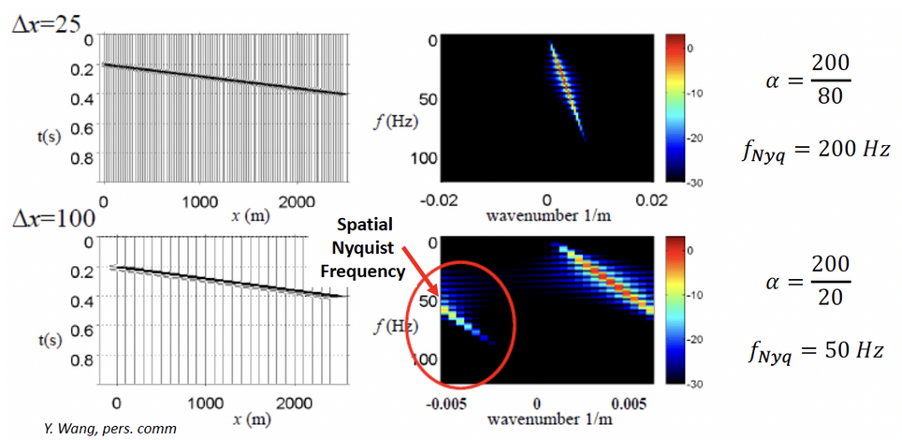
When dealing with gathers in time, we can consider velocity \(v\) as a function of dip (\({\alpha}\), in \(ms\)/trace):
Which combined give:
Wraparound will occur frequencies are higher than the spatial Nyquist frequency
If we consider spatial aliasing in terms of true dip (e.g. in a depth converted stack), then calculating the spatial Nyquist becomes a simple calculation involving velocity \(v\), trace spacing (CMP spacing) \({\Delta}x\) and the dip angle \({\theta}\):
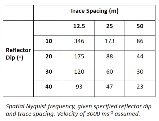
\(12.5\,m\) CMP spacing is relatively safe at even relatively high dips considering the bandwidth of most conventional marine surveys. At larger trace spacing however even relatively small dips are at risk of aliasing across a significant portion of the typical bandwidth. Large sampling interval/trace sapcing or highly dipping events are more prone to spatial aliasing.
Practice 1#
For a linear event in a seismic section, the time dip is measured in terms of milliseconds per trace. A linear dipping event with a slope of \(10\) \(ms\)/trace on a seismic section, at what temporal frequency will the data be spatially aliased?
def f_aliasing(alpha):
    f_nyq = 500/alpha
    return f_nyq

print("At", f_aliasing(10), "Hz will the data be spatially aliased.")
At 50.0 Hz will the data be spatially aliased.
Spatial Aliasing in t-x domain#
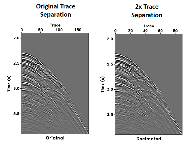
Spatial aliasing can be extremely difficult to identify in the \(t\)-\(x\) domain. Generally, it has a pixelated-like appearance, particularly along steeply dipping events.
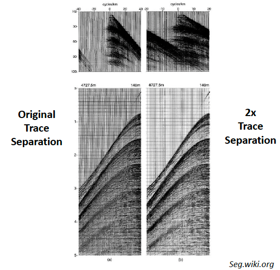
Spatial Aliasing in F-K domain#
Spatial Aliasing is significantly easier to observe in the \(F\)-\(K\) domain, where frequencies above the spatial Nyquist appear as “wrap-around”. We can design a filter to cut out any aliased energy (though this may result in a loss of bandwidth for higher dips) or resample the data at a smaller trace separation (this will make the data volume larger, resulting in more expensive processing). Vice-versa, if there is no spatial aliasing in a dataset, can we increase the trace separation, making further processing cheaper without degrading the image.
In the figure, the CMP gather is highly affected by wraparound with higher trace separation.
Spatial Aliasing and Migration Concerns#
Spatial aliasing is of particular concern when it comes to migration:
Spatially aliased frequencies are perceived by migration to have a different dip to reality
Rather than being relocated to the apex of a hyperbola, these frequencies are dispersed
Also, as migration increases the dip of reflectors, we also have to consider that reflectors could become spatially aliased by migration itself
Reference#
2022 notes and practical from Lecture 6 of the module ESE 60023 Seismic Processing and Lecture 2 of the module ESE 70015 Advance Seismic Processing.