The mixed layer
Contents
The mixed layer#
Geophysical Fluid Dynamics of the Oceans
In this notebook, the mixed layer will be investigated using NetCDF data from the NOAA (National Oceanic and Atmosphereric Administration).
import fsspec
import xarray as xr
The mixed layer is mixed by the winds on the surface creating a homogeneous layer. It is being mixed by wind stress, eddies, kinematic viscosity and convection. The stronger the winds, the deeper the mixed layer. The mixed layer is deeper in the Winter than in Summer. In the Winter, the surface water cooles so it becomes denser causing convection as it is more dense than the layer below. More turbulence also deepens the mixed layer.

The mixed layer is between \(10\) and \(200\,m\) approximately thick depending on stratification (density gradients), season, wind stress, convection and velocity gradient (turbulence and eddies).
To find out more about this dataset, we can evaluate a few factors: You can also try this out for yourself to see how much information is contained in this dataset.
# evaluate the metadata of this Dataset
ocean_data
<xarray.Dataset>
Dimensions:                       (n_param: 3, n_levels: 77, n_history: 4, n_calib: 1)
Dimensions without coordinates: n_param, n_levels, n_history, n_calib
Data variables: (12/65)
    data_type                     object b'Argo profile    '
    format_version                object b'3.1 '
    handbook_version              object b'1.2 '
    reference_date_time           object b'19500101000000'
    date_creation                 object b'20161104225754'
    date_update                   object b'20170714162347'
    ...                            ...
    parameter                     (n_calib, n_param) object b'PRES           ...
    scientific_calib_equation     (n_calib, n_param) object b'PRES_ADJUSTED (...
    scientific_calib_coefficient  (n_calib, n_param) object b'Surface pressur...
    scientific_calib_comment      (n_calib, n_param) object b'Pressure adjust...
    scientific_calib_date         (n_calib, n_param) object b'20170714162348'...
    crs                           int32 -2147483647
Attributes: (12/49)
    title:                           Argo float vertical profile
    institution:                     CORIOLIS
    source:                          Argo float
    history:                         2018-06-09T01:59:23Z csun convAGDAC.f90 ...
    references:                      http://www.nodc.noaa.gov/argo/
    user_manual_version:             3.1
    ...                              ...
    time_coverage_end:               2015-09-07T12:29:26Z
    time_coverage_duration:          point
    time_coverage_resolution:        point
    gadr_ConventionVersion:          GADR-3.0
    gadr_program:                    convAGDAC.f90
gadr_programVersion: 1.0- n_param: 3
- n_levels: 77
- n_history: 4
- n_calib: 1
- data_type()objectb'Argo profile '
- long_name :
- Data type
- conventions :
- Argo reference table 1
array(b'Argo profile ', dtype=object)
- format_version()objectb'3.1 '
- long_name :
- File format version
array(b'3.1 ', dtype=object)
- handbook_version()objectb'1.2 '
- long_name :
- Data handbook version
array(b'1.2 ', dtype=object)
- reference_date_time()objectb'19500101000000'
- long_name :
- Date of reference for Julian days
- conventions :
- YYYYMMDDHHMISS
array(b'19500101000000', dtype=object)
- date_creation()objectb'20161104225754'
- long_name :
- Date of file creation
- conventions :
- YYYYMMDDHHMISS
array(b'20161104225754', dtype=object)
- date_update()objectb'20170714162347'
- long_name :
- Date of update of this file
- conventions :
- YYYYMMDDHHMISS
array(b'20170714162347', dtype=object)
- platform_number()objectb'1901358 '
- long_name :
- Float unique identifier
- conventions :
- WMO float identifier : A9IIIII
array(b'1901358 ', dtype=object)
- project_name()objectb'BSH ...
- long_name :
- Name of the project
array(b'BSH ', dtype=object) - pi_name()objectb'Birgit KLEIN ...
- long_name :
- Name of the principal investigator
array(b'Birgit KLEIN ', dtype=object) - station_parameters(n_param)objectb'PRES ' ... b'PSAL ...
- long_name :
- List of available parameters for the station
- conventions :
- Argo reference table 3
array([b'PRES ', b'TEMP ', b'PSAL '], dtype=object) - cycle_number()float6479.0
- long_name :
- Float cycle number
- conventions :
- 0...N, 0 : launch cycle (if exists), 1 : first complete cycle
array(79.)
- direction()objectb'A'
- long_name :
- Direction of the station profiles
- conventions :
- A: ascending profiles, D: descending profiles
array(b'A', dtype=object)
- data_centre()objectb'IF'
- long_name :
- Data centre in charge of float data processing
- conventions :
- Argo reference table 4
array(b'IF', dtype=object)
- dc_reference()objectb' '
- long_name :
- Station unique identifier in data centre
- conventions :
- Data centre convention
array(b' ', dtype=object)
- data_state_indicator()objectb'2C '
- long_name :
- Degree of processing the data have passed through
- conventions :
- Argo reference table 6
array(b'2C ', dtype=object)
- data_mode()objectb'D'
- long_name :
- Delayed mode or real time data
- conventions :
- R : real time; D : delayed mode; A : real time with adjustment
array(b'D', dtype=object)
- platform_type()objectb'APEX '
- long_name :
- Type of float
- conventions :
- Argo reference table 23
array(b'APEX ', dtype=object)
- float_serial_no()objectb'6459 '
- long_name :
- Serial number of the float
array(b'6459 ', dtype=object)
- firmware_version()objectb'071412 '
- long_name :
- Instrument firmware version
array(b'071412 ', dtype=object)
- wmo_inst_type()objectb'846 '
- long_name :
- Coded instrument type
- conventions :
- Argo reference table 8
array(b'846 ', dtype=object)
- juld()datetime64[ns]2015-09-07T12:29:26.000001024
- long_name :
- Julian day (UTC) of the station relative to REFERENCE_DATE_TIME
- standard_name :
- time
- conventions :
- Relative julian days with decimal part (as parts of day)
- resolution :
- 1.1574074074074073e-05
- axis :
- T
array('2015-09-07T12:29:26.000001024', dtype='datetime64[ns]') - juld_qc()objectb'1'
- long_name :
- Quality on date and time
- conventions :
- Argo reference table 2
array(b'1', dtype=object)
- juld_location()datetime64[ns]2015-09-07T13:48:51.000001024
- long_name :
- Julian day (UTC) of the location relative to REFERENCE_DATE_TIME
- conventions :
- Relative julian days with decimal part (as parts of day)
- resolution :
- 1.9290123456790122e-07
array('2015-09-07T13:48:51.000001024', dtype='datetime64[ns]') - latitude()float64-10.1
- long_name :
- Latitude of the station, best estimate
- standard_name :
- latitude
- units :
- degree_north
- valid_min :
- -90.0
- valid_max :
- 90.0
- axis :
- Y
array(-10.097)
- longitude()float64-3.655
- long_name :
- Longitude of the station, best estimate
- standard_name :
- longitude
- units :
- degree_east
- valid_min :
- -180.0
- valid_max :
- 180.0
- axis :
- X
array(-3.655)
- position_qc()objectb'1'
- long_name :
- Quality on position (latitude and longitude)
- conventions :
- Argo reference table 2
array(b'1', dtype=object)
- positioning_system()objectb'ARGOS '
- long_name :
- Positioning system
array(b'ARGOS ', dtype=object)
- profile_pres_qc()objectb'A'
- long_name :
- Global quality flag of PRES profile
- conventions :
- Argo reference table 2a
array(b'A', dtype=object)
- profile_temp_qc()objectb'A'
- long_name :
- Global quality flag of TEMP profile
- conventions :
- Argo reference table 2a
array(b'A', dtype=object)
- profile_psal_qc()objectb'A'
- long_name :
- Global quality flag of PSAL profile
- conventions :
- Argo reference table 2a
array(b'A', dtype=object)
- vertical_sampling_scheme()objectb'Primary sampling: discrete [] ...
- long_name :
- Vertical sampling scheme
- conventions :
- Argo reference table 16
array(b'Primary sampling: discrete [] ', dtype=object) - config_mission_number()float642.0
- long_name :
- Unique number denoting the missions performed by the float
- conventions :
- 1...N, 1 : first complete mission
array(2.)
- pres(n_levels)float326.2 10.3 15.4 ... 1.9e+03 1.95e+03
- long_name :
- Sea water pressure, equals 0 at sea-level
- standard_name :
- sea_water_pressure
- units :
- decibar
- valid_min :
- 0.0
- valid_max :
- 12000.0
- C_format :
- %7.1f
- FORTRAN_format :
- F7.1
- resolution :
- 0.1
- axis :
- Z
array([ 6.2, 10.3, 15.4, 19.9, 25. , 30.2, 35.5, 40.4, 45.1, 49.7, 60.6, 70.9, 80.2, 90.1, 99.4, 109.4, 119.6, 129.7, 139.6, 149.8, 160. , 170.2, 179.3, 189.7, 199.8, 210.4, 220.6, 230.3, 239.9, 250.2, 260.2, 270.3, 280.5, 289.9, 300. , 310. , 320.3, 330.5, 340.1, 350. , 375.5, 399.6, 424.9, 450.1, 474.8, 549.5, 574.8, 599.9, 625.4, 649.6, 675.6, 700.3, 749.6, 800. , 849. , 900.4, 949.5, 999.4, 1050.1, 1100.3, 1150.6, 1200.5, 1249.8, 1300.3, 1349.9, 1400.2, 1450. , 1500. , 1550.1, 1600.3, 1650. , 1700. , 1750.1, 1800.4, 1850.3, 1899.7, 1950. ], dtype=float32) - pres_qc(n_levels)objectb'1' b'1' b'1' ... b'1' b'1' b'1'
- long_name :
- quality flag
- conventions :
- Argo reference table 2
array([b'1', b'1', b'1', b'1', b'1', b'1', b'1', b'1', b'1', b'1', b'1', b'1', b'1', b'1', b'1', b'1', b'1', b'1', b'1', b'1', b'1', b'1', b'1', b'1', b'1', b'1', b'1', b'1', b'1', b'1', b'1', b'1', b'1', b'1', b'1', b'1', b'1', b'1', b'1', b'1', b'1', b'1', b'1', b'1', b'1', b'1', b'1', b'1', b'1', b'1', b'1', b'1', b'1', b'1', b'1', b'1', b'1', b'1', b'1', b'1', b'1', b'1', b'1', b'1', b'1', b'1', b'1', b'1', b'1', b'1', b'1', b'1', b'1', b'1', b'1', b'1', b'1'], dtype=object) - pres_adjusted(n_levels)float325.8 9.9 15.0 ... 1.899e+03 1.95e+03
- long_name :
- Sea water pressure, equals 0 at sea-level
- standard_name :
- sea_water_pressure
- units :
- decibar
- valid_min :
- 0.0
- valid_max :
- 12000.0
- C_format :
- %7.1f
- FORTRAN_format :
- F7.1
- resolution :
- 0.1
- axis :
- Z
array([ 5.7999997, 9.900001 , 15. , 19.5 , 24.6 , 29.800001 , 35.1 , 40. , 44.699997 , 49.3 , 60.199997 , 70.5 , 79.799995 , 89.7 , 99. , 109. , 119.2 , 129.3 , 139.20001 , 149.40001 , 159.6 , 169.8 , 178.90001 , 189.3 , 199.40001 , 210. , 220.20001 , 229.90001 , 239.5 , 249.8 , 259.80002 , 269.9 , 280.1 , 289.5 , 299.6 , 309.6 , 319.9 , 330.1 , 339.7 , 349.6 , 375.1 , 399.2 , 424.5 , 449.7 , 474.4 , 549.1 , 574.39996 , 599.5 , 625. , 649.19995 , 675.19995 , 699.89996 , 749.19995 , 799.6 , 848.6 , 900. , 949.1 , 999. , 1049.7 , 1099.9 , 1150.2 , 1200.1 , 1249.4 , 1299.9 , 1349.5 , 1399.7999 , 1449.6 , 1499.6 , 1549.7 , 1599.9 , 1649.6 , 1699.6 , 1749.7 , 1800. , 1849.9 , 1899.2999 , 1949.6 ], dtype=float32) - pres_adjusted_qc(n_levels)objectb'1' b'1' b'1' ... b'1' b'1' b'1'
- long_name :
- quality flag
- conventions :
- Argo reference table 2
array([b'1', b'1', b'1', b'1', b'1', b'1', b'1', b'1', b'1', b'1', b'1', b'1', b'1', b'1', b'1', b'1', b'1', b'1', b'1', b'1', b'1', b'1', b'1', b'1', b'1', b'1', b'1', b'1', b'1', b'1', b'1', b'1', b'1', b'1', b'1', b'1', b'1', b'1', b'1', b'1', b'1', b'1', b'1', b'1', b'1', b'1', b'1', b'1', b'1', b'1', b'1', b'1', b'1', b'1', b'1', b'1', b'1', b'1', b'1', b'1', b'1', b'1', b'1', b'1', b'1', b'1', b'1', b'1', b'1', b'1', b'1', b'1', b'1', b'1', b'1', b'1', b'1'], dtype=object) - pres_adjusted_error(n_levels)float322.4 2.4 2.4 2.4 ... 2.4 2.4 2.4 2.4
- long_name :
- Contains the error on the adjusted values as determined by the delayed mode QC process
- units :
- decibar
- C_format :
- %7.1f
- FORTRAN_format :
- F7.1
- resolution :
- 0.1
array([2.4, 2.4, 2.4, 2.4, 2.4, 2.4, 2.4, 2.4, 2.4, 2.4, 2.4, 2.4, 2.4, 2.4, 2.4, 2.4, 2.4, 2.4, 2.4, 2.4, 2.4, 2.4, 2.4, 2.4, 2.4, 2.4, 2.4, 2.4, 2.4, 2.4, 2.4, 2.4, 2.4, 2.4, 2.4, 2.4, 2.4, 2.4, 2.4, 2.4, 2.4, 2.4, 2.4, 2.4, 2.4, 2.4, 2.4, 2.4, 2.4, 2.4, 2.4, 2.4, 2.4, 2.4, 2.4, 2.4, 2.4, 2.4, 2.4, 2.4, 2.4, 2.4, 2.4, 2.4, 2.4, 2.4, 2.4, 2.4, 2.4, 2.4, 2.4, 2.4, 2.4, 2.4, 2.4, 2.4, 2.4], dtype=float32) - temp(n_levels)float3222.74 22.73 22.73 ... 3.453 3.397
- long_name :
- Sea temperature in-situ ITS-90 scale
- standard_name :
- sea_water_temperature
- units :
- degree_Celsius
- valid_min :
- -2.5
- valid_max :
- 40.0
- C_format :
- %9.3f
- FORTRAN_format :
- F9.3
- resolution :
- 0.001
array([22.737, 22.732, 22.729, 22.724, 22.722, 22.721, 22.719, 22.719, 22.719, 22.586, 22.325, 19.672, 18.004, 17.212, 15.692, 14.777, 14.201, 13.593, 13.138, 12.775, 12.222, 11.901, 11.684, 11.577, 11.355, 11.146, 10.965, 10.878, 10.779, 10.6 , 10.528, 10.321, 10.246, 10.11 , 10.053, 9.924, 9.88 , 9.678, 9.584, 9.512, 9.237, 8.896, 8.499, 8.118, 7.801, 7.08 , 6.786, 6.528, 6.306, 6.038, 5.795, 5.582, 5.272, 4.927, 4.67 , 4.444, 4.304, 4.23 , 4.152, 4.099, 4.065, 4.055, 4.026, 3.976, 3.944, 3.915, 3.897, 3.828, 3.784, 3.749, 3.669, 3.619, 3.581, 3.522, 3.49 , 3.453, 3.397], dtype=float32) - temp_qc(n_levels)objectb'1' b'1' b'1' ... b'1' b'1' b'1'
- long_name :
- quality flag
- conventions :
- Argo reference table 2
array([b'1', b'1', b'1', b'1', b'1', b'1', b'1', b'1', b'1', b'1', b'1', b'1', b'1', b'1', b'1', b'1', b'1', b'1', b'1', b'1', b'1', b'1', b'1', b'1', b'1', b'1', b'1', b'1', b'1', b'1', b'1', b'1', b'1', b'1', b'1', b'1', b'1', b'1', b'1', b'1', b'1', b'1', b'1', b'1', b'1', b'1', b'1', b'1', b'1', b'1', b'1', b'1', b'1', b'1', b'1', b'1', b'1', b'1', b'1', b'1', b'1', b'1', b'1', b'1', b'1', b'1', b'1', b'1', b'1', b'1', b'1', b'1', b'1', b'1', b'1', b'1', b'1'], dtype=object) - temp_adjusted(n_levels)float3222.74 22.73 22.73 ... 3.453 3.397
- long_name :
- Sea temperature in-situ ITS-90 scale
- standard_name :
- sea_water_temperature
- units :
- degree_Celsius
- valid_min :
- -2.5
- valid_max :
- 40.0
- C_format :
- %9.3f
- FORTRAN_format :
- F9.3
- resolution :
- 0.001
array([22.737, 22.732, 22.729, 22.724, 22.722, 22.721, 22.719, 22.719, 22.719, 22.586, 22.325, 19.672, 18.004, 17.212, 15.692, 14.777, 14.201, 13.593, 13.138, 12.775, 12.222, 11.901, 11.684, 11.577, 11.355, 11.146, 10.965, 10.878, 10.779, 10.6 , 10.528, 10.321, 10.246, 10.11 , 10.053, 9.924, 9.88 , 9.678, 9.584, 9.512, 9.237, 8.896, 8.499, 8.118, 7.801, 7.08 , 6.786, 6.528, 6.306, 6.038, 5.795, 5.582, 5.272, 4.927, 4.67 , 4.444, 4.304, 4.23 , 4.152, 4.099, 4.065, 4.055, 4.026, 3.976, 3.944, 3.915, 3.897, 3.828, 3.784, 3.749, 3.669, 3.619, 3.581, 3.522, 3.49 , 3.453, 3.397], dtype=float32) - temp_adjusted_qc(n_levels)objectb'1' b'1' b'1' ... b'1' b'1' b'1'
- long_name :
- quality flag
- conventions :
- Argo reference table 2
array([b'1', b'1', b'1', b'1', b'1', b'1', b'1', b'1', b'1', b'1', b'1', b'1', b'1', b'1', b'1', b'1', b'1', b'1', b'1', b'1', b'1', b'1', b'1', b'1', b'1', b'1', b'1', b'1', b'1', b'1', b'1', b'1', b'1', b'1', b'1', b'1', b'1', b'1', b'1', b'1', b'1', b'1', b'1', b'1', b'1', b'1', b'1', b'1', b'1', b'1', b'1', b'1', b'1', b'1', b'1', b'1', b'1', b'1', b'1', b'1', b'1', b'1', b'1', b'1', b'1', b'1', b'1', b'1', b'1', b'1', b'1', b'1', b'1', b'1', b'1', b'1', b'1'], dtype=object) - temp_adjusted_error(n_levels)float320.002 0.002 0.002 ... 0.002 0.002
- long_name :
- Contains the error on the adjusted values as determined by the delayed mode QC process
- units :
- degree_Celsius
- C_format :
- %9.3f
- FORTRAN_format :
- F9.3
- resolution :
- 0.001
array([0.002, 0.002, 0.002, 0.002, 0.002, 0.002, 0.002, 0.002, 0.002, 0.002, 0.002, 0.002, 0.002, 0.002, 0.002, 0.002, 0.002, 0.002, 0.002, 0.002, 0.002, 0.002, 0.002, 0.002, 0.002, 0.002, 0.002, 0.002, 0.002, 0.002, 0.002, 0.002, 0.002, 0.002, 0.002, 0.002, 0.002, 0.002, 0.002, 0.002, 0.002, 0.002, 0.002, 0.002, 0.002, 0.002, 0.002, 0.002, 0.002, 0.002, 0.002, 0.002, 0.002, 0.002, 0.002, 0.002, 0.002, 0.002, 0.002, 0.002, 0.002, 0.002, 0.002, 0.002, 0.002, 0.002, 0.002, 0.002, 0.002, 0.002, 0.002, 0.002, 0.002, 0.002, 0.002, 0.002, 0.002], dtype=float32) - psal(n_levels)float3236.35 36.35 36.35 ... 34.93 34.93
- long_name :
- Practical salinity
- standard_name :
- sea_water_salinity
- units :
- psu
- valid_min :
- 2.0
- valid_max :
- 41.0
- C_format :
- %9.3f
- FORTRAN_format :
- F9.3
- resolution :
- 0.001
array([36.347, 36.346, 36.347, 36.347, 36.346, 36.347, 36.347, 36.347, 36.346, 36.371, 36.464, 36.216, 35.998, 35.904, 35.7 , 35.574, 35.488, 35.41 , 35.343, 35.29 , 35.214, 35.166, 35.135, 35.121, 35.091, 35.063, 35.042, 35.03 , 35.017, 34.997, 34.988, 34.965, 34.955, 34.942, 34.934, 34.921, 34.914, 34.893, 34.885, 34.875, 34.846, 34.81 , 34.771, 34.735, 34.707, 34.643, 34.619, 34.6 , 34.584, 34.566, 34.55 , 34.536, 34.52 , 34.511, 34.513, 34.531, 34.559, 34.588, 34.617, 34.658, 34.692, 34.716, 34.748, 34.787, 34.816, 34.846, 34.861, 34.878, 34.895, 34.909, 34.916, 34.921, 34.923, 34.926, 34.927, 34.928, 34.929], dtype=float32) - psal_qc(n_levels)objectb'1' b'1' b'1' ... b'1' b'1' b'1'
- long_name :
- quality flag
- conventions :
- Argo reference table 2
array([b'1', b'1', b'1', b'1', b'1', b'1', b'1', b'1', b'1', b'1', b'1', b'1', b'1', b'1', b'1', b'1', b'1', b'1', b'1', b'1', b'1', b'1', b'1', b'1', b'1', b'1', b'1', b'1', b'1', b'1', b'1', b'1', b'1', b'1', b'1', b'1', b'1', b'1', b'1', b'1', b'1', b'1', b'1', b'1', b'1', b'1', b'1', b'1', b'1', b'1', b'1', b'1', b'1', b'1', b'1', b'1', b'1', b'1', b'1', b'1', b'1', b'1', b'1', b'1', b'1', b'1', b'1', b'1', b'1', b'1', b'1', b'1', b'1', b'1', b'1', b'1', b'1'], dtype=object) - psal_adjusted(n_levels)float3236.35 36.35 36.35 ... 34.93 34.93
- long_name :
- Practical salinity
- standard_name :
- sea_water_salinity
- units :
- psu
- valid_min :
- 2.0
- valid_max :
- 41.0
- C_format :
- %9.3f
- FORTRAN_format :
- F9.3
- resolution :
- 0.001
array([36.347137, 36.346138, 36.347137, 36.347137, 36.346138, 36.347137, 36.347137, 36.347137, 36.346138, 36.371136, 36.46414 , 36.21615 , 35.998154, 35.904156, 35.700222, 35.574207, 35.488194, 35.41019 , 35.34318 , 35.290184, 35.21418 , 35.16618 , 35.135178, 35.121178, 35.09118 , 35.06318 , 35.04218 , 35.030178, 35.017178, 34.99718 , 34.98818 , 34.96518 , 34.955185, 34.942184, 34.93418 , 34.921185, 34.914185, 34.893185, 34.88518 , 34.875187, 34.846188, 34.810192, 34.771194, 34.735195, 34.7072 , 34.643208, 34.61921 , 34.60021 , 34.584213, 34.56622 , 34.550217, 34.53622 , 34.52022 , 34.511227, 34.513226, 34.53122 , 34.55922 , 34.58822 , 34.617214, 34.658215, 34.69221 , 34.716206, 34.748207, 34.7872 , 34.816204, 34.8462 , 34.8612 , 34.878197, 34.8952 , 34.909195, 34.916195, 34.921196, 34.923195, 34.926193, 34.927193, 34.928196, 34.92919 ], dtype=float32) - psal_adjusted_qc(n_levels)objectb'1' b'1' b'1' ... b'1' b'1' b'1'
- long_name :
- quality flag
- conventions :
- Argo reference table 2
array([b'1', b'1', b'1', b'1', b'1', b'1', b'1', b'1', b'1', b'1', b'1', b'1', b'1', b'1', b'1', b'1', b'1', b'1', b'1', b'1', b'1', b'1', b'1', b'1', b'1', b'1', b'1', b'1', b'1', b'1', b'1', b'1', b'1', b'1', b'1', b'1', b'1', b'1', b'1', b'1', b'1', b'1', b'1', b'1', b'1', b'1', b'1', b'1', b'1', b'1', b'1', b'1', b'1', b'1', b'1', b'1', b'1', b'1', b'1', b'1', b'1', b'1', b'1', b'1', b'1', b'1', b'1', b'1', b'1', b'1', b'1', b'1', b'1', b'1', b'1', b'1', b'1'], dtype=object) - psal_adjusted_error(n_levels)float320.01 0.01 0.01 ... 0.01 0.01 0.01
- long_name :
- Contains the error on the adjusted values as determined by the delayed mode QC process
- units :
- psu
- C_format :
- %9.3f
- FORTRAN_format :
- F9.3
- resolution :
- 0.001
array([0.01, 0.01, 0.01, 0.01, 0.01, 0.01, 0.01, 0.01, 0.01, 0.01, 0.01, 0.01, 0.01, 0.01, 0.01, 0.01, 0.01, 0.01, 0.01, 0.01, 0.01, 0.01, 0.01, 0.01, 0.01, 0.01, 0.01, 0.01, 0.01, 0.01, 0.01, 0.01, 0.01, 0.01, 0.01, 0.01, 0.01, 0.01, 0.01, 0.01, 0.01, 0.01, 0.01, 0.01, 0.01, 0.01, 0.01, 0.01, 0.01, 0.01, 0.01, 0.01, 0.01, 0.01, 0.01, 0.01, 0.01, 0.01, 0.01, 0.01, 0.01, 0.01, 0.01, 0.01, 0.01, 0.01, 0.01, 0.01, 0.01, 0.01, 0.01, 0.01, 0.01, 0.01, 0.01, 0.01, 0.01], dtype=float32) - history_institution(n_history)objectb'IF ' b'IF ' b'IF ' b'GE '
- long_name :
- Institution which performed action
- conventions :
- Argo reference table 4
array([b'IF ', b'IF ', b'IF ', b'GE '], dtype=object)
- history_step(n_history)objectb'ARFM' b'ARGQ' b'ARGQ' b'ARSQ'
- long_name :
- Step in data processing
- conventions :
- Argo reference table 12
array([b'ARFM', b'ARGQ', b'ARGQ', b'ARSQ'], dtype=object)
- history_software(n_history)objectb'CODA' b'COQC' b'COQC' b'OW '
- long_name :
- Name of software which performed action
- conventions :
- Institution dependent
array([b'CODA', b'COQC', b'COQC', b'OW '], dtype=object)
- history_software_release(n_history)objectb'008a' b'2.7 ' b'2.7 ' b'1.0 '
- long_name :
- Version/release of software which performed action
- conventions :
- Institution dependent
array([b'008a', b'2.7 ', b'2.7 ', b'1.0 '], dtype=object)
- history_reference(n_history)objectb' ...
- long_name :
- Reference of database
- conventions :
- Institution dependent
array([b' ', b' ', b' ', b'ARGO CTD ref. database: CTD_for_DMQC_2016V01 + ARGO climatology '], dtype=object) - history_date(n_history)objectb'20161104225754' ... b'20170714...
- long_name :
- Date the history record was created
- conventions :
- YYYYMMDDHHMISS
array([b'20161104225754', b'20161104225824', b'20161104225824', b'20170714162348'], dtype=object) - history_action(n_history)objectb' ' b'QCP$' b'QCF$' b'IP '
- long_name :
- Action performed on data
- conventions :
- Argo reference table 7
array([b' ', b'QCP$', b'QCF$', b'IP '], dtype=object)
- history_parameter(n_history)objectb' ' ... b'PSAL ...
- long_name :
- Station parameter action is performed on
- conventions :
- Argo reference table 3
array([b' ', b' ', b' ', b'PSAL '], dtype=object) - history_start_pres(n_history)float32nan nan nan 6.2
- long_name :
- Start pressure action applied on
- units :
- decibar
array([nan, nan, nan, 6.2], dtype=float32)
- history_stop_pres(n_history)float32nan nan nan 1.95e+03
- long_name :
- Stop pressure action applied on
- units :
- decibar
array([ nan, nan, nan, 1950.], dtype=float32)
- history_previous_value(n_history)float32nan nan nan nan
- long_name :
- Parameter/Flag previous value before action
array([nan, nan, nan, nan], dtype=float32)
- history_qctest(n_history)objectb' ' ... b' ...
- long_name :
- Documentation of tests performed, tests failed (in hex form)
- conventions :
- Write tests performed when ACTION=QCP$; tests failed when ACTION=QCF$
array([b' ', b'000000000008FB7E', b'0000000000000000', b' '], dtype=object) - parameter(n_calib, n_param)objectb'PRES ' ... b'PSAL ...
- long_name :
- List of parameters with calibration information
- conventions :
- Argo reference table 3
array([[b'PRES ', b'TEMP ', b'PSAL ']], dtype=object) - scientific_calib_equation(n_calib, n_param)objectb'PRES_ADJUSTED (cycle i) = PRES...
- long_name :
- Calibration equation for this parameter
array([[b'PRES_ADJUSTED (cycle i) = PRES (cycle i) - Surface Pressure (cycle i+1) ', b'TEMP_ADJUSTED = TEMP ', b'PSAL_ADJUSTED = PSAL (re-calculated by using PRES_ADJUSTED) ']], dtype=object) - scientific_calib_coefficient(n_calib, n_param)objectb'Surface pressure = 0.4 dbar ...
- long_name :
- Calibration coefficients for this equation
array([[b'Surface pressure = 0.4 dbar ', b'none ', b'none ']], dtype=object) - scientific_calib_comment(n_calib, n_param)objectb'Pressure adjusted by using pre...
- long_name :
- Comment applying to this parameter calibration
array([[b'Pressure adjusted by using pressure offset at the sea surface. Calibration error is manufacturer specified accuracy in dbar ', b'No significant temperature drift detected. Calibration error is manufacturer specified accuracy with respect to ITS-90 ', b'No significant salinity drift detected (salinity adjusted for pressure offset). OW method (weighted least squares fit) adopted. The quoted error is max[0.01, 1xOW uncertainty] in PSS-78. ']], dtype=object) - scientific_calib_date(n_calib, n_param)objectb'20170714162348' ... b'20170714...
- long_name :
- Date of calibration
- conventions :
- YYYYMMDDHHMISS
array([[b'20170714162348', b'20170714162348', b'20170714162348']], dtype=object) - crs()int32-2147483647
- long_name :
- Coordinate Reference System
- grid_mapping_name :
- latitude_longitude
- epsg_code :
- EPSG:4326
- longitude_of_prime_meridian :
- 0.0f
- semi_major_axis :
- 6378137.0
- inverse_flattening :
- 298.257223563
array(-2147483647, dtype=int32)
- title :
- Argo float vertical profile
- institution :
- CORIOLIS
- source :
- Argo float
- history :
- 2018-06-09T01:59:23Z csun convAGDAC.f90 Version 1.0
- references :
- http://www.nodc.noaa.gov/argo/
- user_manual_version :
- 3.1
- Conventions :
- GADR-3.0 Argo-3.0 CF-1.6
- featureType :
- trajectoryProfile
- uuid :
- 6a5c9705-6b09-4528-9ca2-e8efd6fc78db
- summary :
- The U.S. National Oceanographic Data Center (NODC) operates the Argo Global Data Repository (GADR). For information about organizations contributing data to GADR, see http://www.nodc.noaa.gov/argo/
- file_source :
- The Argo Global Data Assembly Center FTP server at ftp://ftp.ifremer.fr/ifremer/argo
- keywords :
- temperature, salinity, sea_water_temperature, sea_water_salinity
- keywords_vocabulary :
- NODC Data Types, CF Standard Names
- creator_name :
- Charles Sun
- creator_url :
- http://www.nodc.noaa.gov
- creator_email :
- Charles.Sun@noaa.gov
- id :
- 0042682
- naming_authority :
- gov.noaa.nodc
- standard_name_vocabulary :
- CF-1.6
- Metadata_Conventions :
- Unidata Dataset Discovery v1.0
- publisher_name :
- US DOC; NESDIS; NATIONAL OCEANOGRAPHIC DATA CENTER - IN295
- publisher_url :
- http://www.nodc.noaa.gov/
- publisher_email :
- NODC.Services@noaa.gov
- date_created :
- 2018-06-09T01:59:23Z
- date_modified :
- 2018-06-09T01:59:23Z
- date_issued :
- 2018-06-09T01:59:23Z
- acknowledgment :
- These data were acquired from the US NOAA National Oceanographic Data Center (NODC) on [DATE] from http://www.nodc.noaa.gov/.
- license :
- These data are openly available to the public Please acknowledge the use of these data with the text given in the acknowledgment attribute.
- cdm_data_type :
- trajectoryProfile
- geospatial_lat_min :
- -10.097
- geospatial_lat_max :
- -10.097
- geospatial_lon_min :
- -3.655
- geospatial_lon_max :
- -3.655
- geospatial_vertical_min :
- 6.2
- geospatial_vertical_max :
- 1950.0
- geospatial_lat_units :
- degrees_north
- geospatial_lat_resolution :
- point
- geospatial_lon_units :
- degrees_east
- geospatial_lon_resolution :
- point
- geospatial_vertical_units :
- decibars
- geospatial_vertical_resolution :
- point
- geospatial_vertical_positive :
- down
- time_coverage_start :
- 2015-09-07T12:29:26Z
- time_coverage_end :
- 2015-09-07T12:29:26Z
- time_coverage_duration :
- point
- time_coverage_resolution :
- point
- gadr_ConventionVersion :
- GADR-3.0
- gadr_program :
- convAGDAC.f90
- gadr_programVersion :
- 1.0
print('The location of this dataset is at (', ocean_data['longitude'].data,',', ocean_data['latitude'].data, ')')
print('The minimum value of temperature in this part of the ocean is', min(ocean_data['temp'].data), 'deg Celcius')
print('The maximum value of temperature in this part of the ocean is', max(ocean_data['temp'].data), 'deg Celcius')
The location of this dataset is at ( -3.6549999999999727 , -10.097 )
The minimum value of temperature in this part of the ocean is 3.397 deg Celcius
The maximum value of temperature in this part of the ocean is 22.737 deg Celcius
fig, ax = plt.subplots(ncols=2, figsize=(15,6))

fig.suptitle('Temperature and salinity at depth with increasing pressure', fontsize=16)

ocean_data.temp.plot(y='n_levels', ax=ax[0], yincrease=False, label='T')
ocean_data.psal.plot(y='n_levels', ax=ax[1], yincrease=False, label='Salinity')

ax[0].legend()
ax[1].legend()

ax[0].set_xlabel('Sea temperature in [$\deg C $]')
ax[0].set_ylabel('Depth from surface in number of levels')
ax[1].set_xlabel('Practical Salinity in [g/kg]')
ax[1].set_ylabel('Depth from surface in number of levels')
Text(0, 0.5, 'Depth from surface in number of levels')
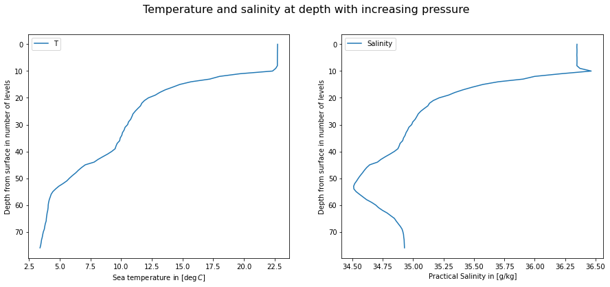
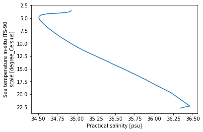
From the above plots, it can be seen that temperature and salinity look homogeneous in the mixed layer. Below the mixed layer is the thermocline which is a region where the temperature gradient is very steep. The termocline is between \(300\) and \(1000\,m\) and is steepest for example in the Artic where fresh cold water overlies warmer watter.
Temperature-salinity relationship#
Next, a temperature-salinity profile can be plotted that is independent of depth.
# swap dimensions to temperature data
ocean_data_temp = argo.swap_dims({'n_levels': 'temp'})
ocean_data_temp.psal.plot(y='temp', yincrease=False, label='Practical salinity')
[<matplotlib.lines.Line2D at 0x7f91802e6a90>]