1D heat conduction (layered medium)

Geodynamics

1D steady state heat equation

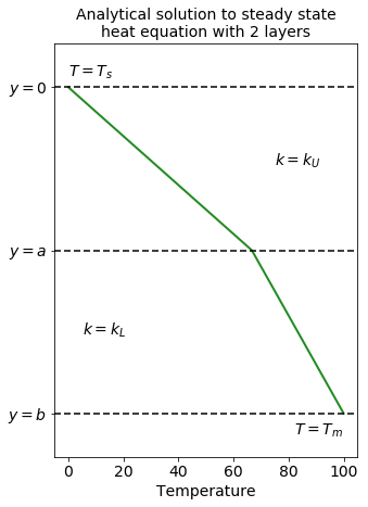
Consider a 1D model with two layers of different thermal conductivities - \(k_U\) for layer \(0 < y < a\) and \(k_L\) for layer \(a < y < b\). In either layer, no heat is generated.

Boundary conditions:

• temperature at \(y=0\) is \(T_s\)

• temperature at \(y=b\) is \(T_m\)

The governing ODE for each layer is:

\[k\frac{d^2T}{dy^2}=0.\]

Analytical solution

Analytically, the ODE can be solved separately for upper and lower layer.

Upper layer ODE can be written as

\[k_U\frac{d^2 T_U}{dy^2}=0.\]

Integrating ODE once with respect to \(y\) we obtain

\[\frac{dT_U}{dy}=A,\]

where \(A\) is a constant of integration. Integrating once again, we get

\[T_U(y) = Ay+B.\]

Now, using boundary condition at \(y=0\):

\[T_U(0)=A\times 0 + B =T_s\Rightarrow B = T_s,\]

\[T_U(y)=Ay+T_s.\]

Similarly for lower layer ODE is

\[k_L\frac{d^2 T_L}{dy^2}=0 \Rightarrow T_L(y)=Cy+D.\]

Using boundary condition at \(y=b\), we get:

\[T_L(b)=Cb+D=T_m\Rightarrow D=T_m-Cb,\]

\[T_L(y)=T_m+C(y-b).\]

We have two unknown constants \(A\) and \(C\). For that, we need two more boundary conditions:

• temperature is continuous at the interface:

  \[T_L(a)=T_U(a)\]

• heat flux is continuous at the interface

The first condition yields:

\[Aa+T_s=T_m+C(a-b),\]

\[A=\frac{T_m-T_s+C(a-b)}{a}.\]

The solutions for both layers are then:

\[T_U =T_s+[T_m-T_s+C(a-b)]\frac{y}{a},\]

\[T_L = T_m+C(y-b).\]

The upwards heat flux into the interface from the lower layer is:

\[k_L\frac{dT_U(y)}{dy}\Big|_{y=a}=k_LC.\]

The upwards heat flux away from the interface into the upper layer is:

\[k_U\frac{dT_L(y)}{dy}\Big|_{y=a}=k_U[T_m-T_s+C(a-b)].\]

Equating these two heat fluxes we get:

\[k_LC=k_U[T_m-T_s+C(a-b)],\]

\[C=\frac{k_U(T_m-T_s)}{ak_L+(b-a)k_U}.\]

Therefore, the analytical solution yields:

\[T_U = T_s + (T_m-T_s) \Big[\frac{k_L}{ak_L +(b-a)k_U}\Big] y,\]

\[T_L = T_m + (T_m-T_s) \Big[\frac{k_U}{ak_L +(b-a)k_U}\Big] (y-b).\]

We can calculate and plot the analytical solution with the following code:

import matplotlib.pyplot as plt
import numpy as np

# Set boundary temperature
T_s = 0
T_m = 100

# Set y 
N = 51
L = 30
y = np.linspace(0,L,N)

# Set thermal conductivities
k_upper = 1
k_lower = 2

# Set layer thickness
a = y[int(N/2)]
b = y[-1]

# Calculate tempearture profile
T = np.zeros(N)

for i in range(len(T)):
    if y[i] <= a:
        T[i] = T_s+(T_m-T_s)*(k_lower/(a*k_lower+(b-a)*k_upper))*y[i]
    else:
        T[i] = T_m +(T_m-T_s)*(k_upper/(a*k_lower+(b-a)*k_upper))*(y[i]-b)

plt.figure(figsize=(5,7))

plt.plot(T, -y, color="forestgreen", lw=2)

plt.axhline(0, color="black", dashes=(4,2))
plt.axhline(-y[int(N/2)], color="black", dashes=(4,2))
plt.axhline(-y[-1], color="black", dashes=(4,2))

plt.xlabel("Temperature", fontsize=14)

plt.yticks([0, -y[int(N/2)], -y[-1]], ["$y=0$", "$y=a$", "$y=b$"], fontsize=14)
plt.xticks(fontsize=14)

plt.text(T[-1]*3/4., -y[int(N/4)], "$k=k_U$", fontsize=14)
plt.text(T[0]+5, -y[int(3*N/4)], "$k=k_L$", fontsize=14)
plt.text(T[0], -y[0]+1, "$T=T_s$", fontsize=14)
plt.text(T[-1], -y[-1]-2, "$T=T_m$", fontsize=14, ha='right')

plt.ylim(-y[-1]-4, -y[0]+4)
plt.xlim(T[0]-5, T[-1]+5)

plt.title("Analytical solution to steady state\nheat equation with 2 layers",
         fontsize=14)

plt.show()

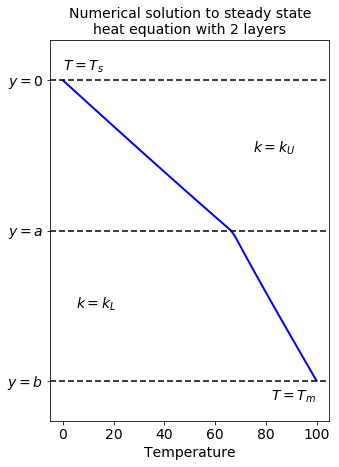
Numerical solution

In the previous section, we showed how to analytically solve 1D steady state heat equation for two layers with different thermal conductivities. Next, we will create a numerical solution.

Discretisation

The steady state ODE for heat equation in one dimension for material with uniform thermal conductivity states:

\[k\frac{d^2T}{dy^2}=0.\]

However, since our model has two layers of different conductivities, the equation becomes instead:

\[\frac{\partial}{\partial y}\Big(k\frac{\partial T}{\partial x}\Big)=0.\]

Thermal conductivity

Thermal conductivity \(k\) in this example is a piece-wise constant, therefore

\[\frac{dk}{dx}\]

is a delta function. In the present case, our boundary conditions lead to the term

\[\frac{(k_{i+1}-k_{i-1})}{8k_i}(T_{i+1}-T_{i-1})\]

beging much smaller than

\[\frac{1}{2}(T_{i+1}+T_{i-1})\]

term. However, if the changes in conductivity were of several orders of magnitude, discretising this problem with finite difference would be very difficult!

Using chain rule, we obtain:

\[\frac{\partial k}{\partial y}\frac{\partial T}{\partial y}+k\frac{\partial^2T}{\partial y^2} =0.\]

To discretise the equation, we will use finite difference methods. First derivative of temperature and thermal conductivity are described as

\[\left(\frac{\partial T}{\partial y} \right)\bigg\rvert_{y=y_i} \approx\frac{T_{i+1}-T_{i-1}}{2\Delta y}, \quad \left(\frac{\partial k}{\partial y}\right) \bigg\rvert_{y=y_i} \approx\frac{k_{i+1}-k_{i-1}}{2\Delta y}.\]

The second derivative of temperature is

\[\left(\frac{\partial^2 T}{\partial y^2}\right)\bigg\rvert_{y=y_i}\approx\frac{T_{i+1}-2T_{i}+T_{i-1}}{(\Delta y)^2}.\]

Now, we can substitude these into our equation:

\[\frac{k_{i+1}-k_{i-1}}{2\Delta y}\frac{T_{i+1}-T_{i-1}}{2\Delta y}+k_i\frac{T_{i+1}-2T_{i}+T_{i-1}}{(\Delta y)^2}=0\quad ||\cdot 4(\Delta y)^2,\]

\[(k_{i+1}-k_{i-1})(T_{i+1}-T_{i-1})+4k_i(T_{i+1}-2T_i+T_{i-1})=0,\]

\[8k_i T_i = (k_{i+1}-k_{i-1})(T_{i+1}-T_{i-1}) +4k_i(T_{i+1}+T_{i-1}).\]

And finally, we obtain the solution for temperature at \(y_i\):

\[T_i = \frac{(k_{i+1}-k_{i-1})}{8k_i}(T_{i+1}-T_{i-1}) +\frac{1}{2}(T_{i+1}+T_{i-1}).\]

Code below shows the implementation and plot of obtained temperature profile:

# Set temperature arrays
T_old = np.zeros(N)
T_new = np.zeros(N)

# Set boundary conditions
T_old[0] = T_s
T_old[-1] = T_m

# Create y array
y = np.linspace(0,L,N)

# Create k array and 
# substitute correct conductivities
k = np.zeros(N)

for i in range(len(k)):
    if i <= int(N/2):
        k[i] = k_upper
    else:
        k[i] = k_lower

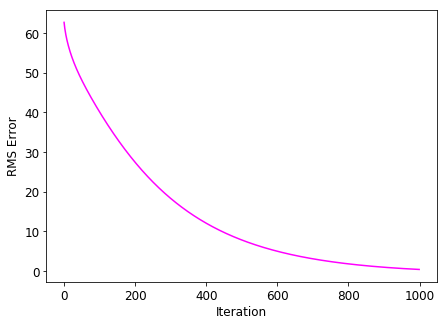
To obtain the temperature profile, we need to update \(T_{old}\) multiple times to make sure our steady state solution converged. We will use RMS error to see how our solution converges as compared to the analytical solution:

from sklearn.metrics import mean_squared_error

nf = 1000

rms = np.zeros(nf)

for it in range(nf):
    
    T_new = T_old

    for i in range(1,N-1):
        T_new[i] = (k[i+1]-k[i-1])/(8*k[i])*(T_old[i+1]-T_old[i-1])+1./2.*(T_old[i+1]+T_old[i-1])
        
    rms[it] = np.sqrt(mean_squared_error(T, T_new))
    
plt.figure(figsize=(7,5))
plt.plot(rms, color="magenta")
plt.xticks(fontsize=12)
plt.yticks(fontsize=12)
plt.xlabel("Iteration", fontsize=12)
plt.ylabel("RMS Error", fontsize=12)
plt.show()

Now we can plot the numerical solution:

plt.figure(figsize=(5,7))

plt.plot(T_new, -y, color="blue", lw=2)

plt.axhline(0, color="black", dashes=(4,2))
plt.axhline(-y[int(N/2)], color="black", dashes=(4,2))
plt.axhline(-y[-1], color="black", dashes=(4,2))

plt.xlabel("Temperature", fontsize=14)

plt.yticks([0, -y[int(N/2)], -y[-1]], ["$y=0$", "$y=a$", "$y=b$"], fontsize=14)
plt.xticks(fontsize=14)

plt.text(T_old[-1]*3/4., -y[int(N/4)], "$k=k_U$", fontsize=14)
plt.text(T_old[0]+5, -y[int(3*N/4)], "$k=k_L$", fontsize=14)
plt.text(T_old[0], -y[0]+1, "$T=T_s$", fontsize=14)
plt.text(T_old[-1], -y[-1]-2, "$T=T_m$", fontsize=14, ha='right')

plt.ylim(-y[-1]-4, -y[0]+4)
plt.xlim(T_old[0]-5, T_old[-1]+5)

plt.title("Numerical solution to steady state\nheat equation with 2 layers",
         fontsize=14)

plt.show()

Numerical vs. analytical solution

To compare the solutions, we will plot them and their difference at the same graph:

fig, axes = plt.subplots(1, 2, figsize=(8,6),
                        sharey=True)

ax1 = axes[0]
ax2 = axes[1]

ax1.plot(T, -y, color="forestgreen", dashes=(4,2),
         lw=3, label="Analytical solution", zorder=2)

ax1.plot(T_new, -y, color="blue", dashes=(6,2),
         lw=3, label="Numerical solution", zorder=1)

ax1.legend(loc="best", fontsize=12)

ax1.set_xlabel("Temperature", fontsize=12)
ax1.set_ylabel("Depth", fontsize=12)


ax2.plot(T_new-T, -y, color="magenta",
        lw=2, label="$T_{num}-T_{analytical}$")

ax2.set_xlabel("Residual temperature",
              fontsize=12)

ax2.legend(loc="best", fontsize=12)

# Create root mean scquared error
rms = np.sqrt(mean_squared_error(T, T_new))

ax2.set_title("RMS Error = %.4f" % rms)

plt.show()

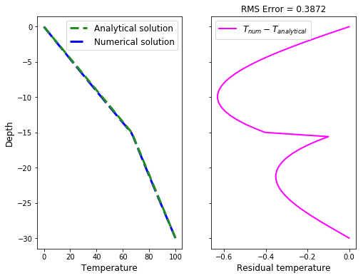
As we can see on the graphs, the numerical solution is very close to the analytical solution.

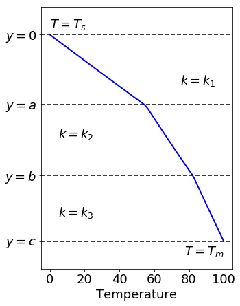
Three layers

The same numerical analysis can be applied to multiple layers with different thermal conductivites. Here we show an example of three layer model:

Setup the model

N = 51
L = 30
T_old = np.zeros(N)
T_new = np.zeros(N)

T_old[0] = 0.
T_old[-1] = 100.

y = np.linspace(0,L,N)
k = np.zeros(N)

k1= 1
k2 = 2
k3 = 3
l1 = y[int(N/3)]
l2 = y[int(2*N/3)]
l3 = y[int(N)-1]

for i in range(len(k)):
    if y[i] <= l1:
        k[i] = k1
    elif y[i] <= l2:
        k[i] = k2
    else:
        k[i] = k3

Run the steady state solution

nf = 1000
for it in range(nf):
    
    T_new = T_old

    for i in range(1,N-1):
        T_new[i] = (k[i+1]-k[i-1])/(8*k[i])*(T_old[i+1]-T_old[i-1])+1./2.*(T_old[i+1]+T_old[i-1])
        

Plot the results

plt.figure(figsize=(5,7))

plt.plot(T_new, -y, color="blue", lw=2)

plt.axhline(0, color="black", dashes=(4,2))
plt.axhline(-y[int(N/3)], color="black", dashes=(4,2))
plt.axhline(-y[int(2*N/3)], color="black", dashes=(4,2))
plt.axhline(-y[-1], color="black", dashes=(4,2))

plt.xlabel("Temperature", fontsize=18)

plt.yticks([0, -y[int(N/3)],-y[int(2*N/3)], -y[-1]],
        ["$y=0$", "$y=a$", "$y=b$", "$y=c$"], fontsize=18)
plt.xticks(fontsize=18)

plt.text(T_old[-1]*3/4., -y[int(N/4)], "$k=k_1$", fontsize=18)
plt.text(T_old[0]+5, -y[int(N/2)], "$k=k_2$", fontsize=18)
plt.text(T_old[0]+5, -y[int(7*N/8)], "$k=k_3$", fontsize=18)
plt.text(T_old[0], -y[0]+1, "$T=T_s$", fontsize=18)
plt.text(T_old[-1], -y[-1]-2, "$T=T_m$", fontsize=18, ha='right')

plt.ylim(-y[-1]-4, -y[0]+4)
plt.xlim(T_old[0]-5, T_old[-1]+5)

plt.show()

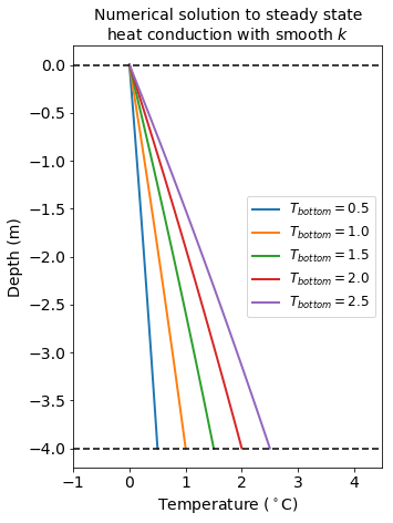
Smooth k

So far, we created a piece wise function of thermal conductivity. In real life, it is more often the case that \(k\) varies smoothly in space, especially at shallow depths.

Fisher et al. (2001) provides a relationship between depth and thermal conductivity for top \(4\,m\) in the Alarcon basin based on field survey:

\[k = 0.70 + 0.0035\times \text{depth}.\]

According, to Figure 2 from the paper, we could take top temperature at \(0^\circ C\) and bottom temperature between \(0.5^\circ C\) and \(2.5^\circ C\).

Try writing the code yourself!!

You will need to:

1. Make a list of bottom temperatures

2. Loop over the list to create temperature profiles

3. Plot the profiles

The numerical solution for these temperatures then looks:

References

• Material used in this notebook was based on lecture content of Geodynamics module at Earth Science and Engineering Department at Imperial College London

• Fisher, A.T., Giambalvo, E., Sclater, J., Kastner, M., Ransom, B., Weinstein, Y. and Lonsdale, P., 2001. Heat flow, sediment and pore fluid chemistry, and hydrothermal circulation on the east flank of Alarcon Ridge, Gulf of California. Earth and Planetary Science Letters, 188(3-4), pp.521-534.