Impedance, Transmission and Reflection

Waves

In this chapter, impedance, reflection and transmission will be discussed.

import numpy as np
import matplotlib.pyplot as plt

Impedance

Impedance is a measure of how difficult it is for a wave to travel through a certain medium.

The physical properties characterizing the model are density (\(\rho\)) and seismic velocity (\(c\))

The acoustic impedance of each layer is:

\[ Z = \rho c \]

with units \([kg\,s^{-1}]\).

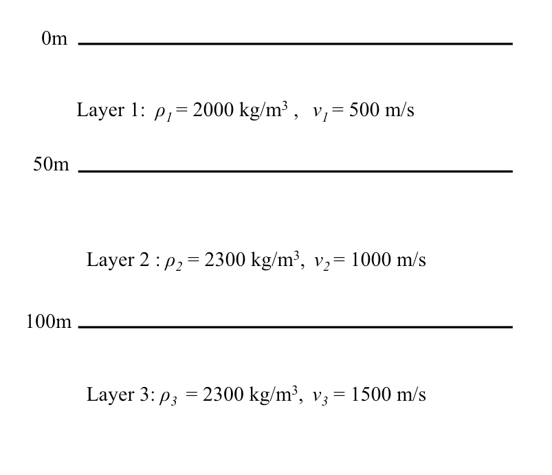
Consider a reflectivity model and let’s calculate the impedance for all three layers.

def acoustic_impedance(rho, c, layer_number):
    z = rho*c
    print('The acoustic impedance of layer', layer_number, '=', z, 'kg/s')
    return z

rho1 = 2000
v1 = 500
rho2 = 2300
v2 = 1000
rho3 = 2300
v3 = 1500

z1 = acoustic_impedance(rho1, v1, 1)
z2 = acoustic_impedance(rho2, v2, 2)
z3 = acoustic_impedance(rho3, v3, 3)

The acoustic impedance of layer 1 = 1000000 kg/s
The acoustic impedance of layer 2 = 2300000 kg/s
The acoustic impedance of layer 3 = 3450000 kg/s

It can thus be seen that a higher seismic velocity results in a higher impedance and thus easier passage for the wave. This is similar for a higher density.

Reflection and Transmission

Reflection and Transmission (Transverse waves)

Consider acoustic impedance in a different light where a seismic wave travels through a medium. When an incident wave apporaches a boundary of different density and seismic velocity (thus, different impedance), a wave can reflected or transmitted. We make a few assumptions:

• \(y_i + y_r = y_p\) (for a continuous string across a boundary and conservation of energy)

• tension in the string must be continuous

Consider the subscript \(i\) for the incidence wave, \(r\) for the reflected wave and \(p\) for the propagating/transmitted wave.

Consider coefficients of reflection and transmission now as the ratio between the amplitude of the reflected/transmitted wave and incident wave respectively.

The reflection coefficient is

\[ R = \frac{y_{0r}}{y_{0i}}\]

and the transmission coefficient is

\[ P = \frac{y_{0p}}{y_{0i}}\]

For this module, we are assuming that the incident wave travels normal to the boundary. Thus \(\theta_i = \theta_r = \theta_p = 0\).

From acoustic impedance, the down-going reflection coefficient for amplitude is given by

\[ R = \frac{Z_{1}-Z_2}{Z_1+Z_2} \]

and the transmission coefficient is

\[ P = \frac{2Z_{1}}{Z_1+Z_2} \]

Considering wave energy transfer, where wave total energy per unit string is defined as \( E = \frac{ \rho \omega^2 {y_0}^2}{2}\).

\[ R = \left(\frac{Z_{1}-Z_2}{Z_1+Z_2}\right)^2 \]

\[ P = \frac{4 Z_{1} Z_2}{(Z_1+Z_2)^2} \]

Note that 1 + R = P always, from conservation of energy

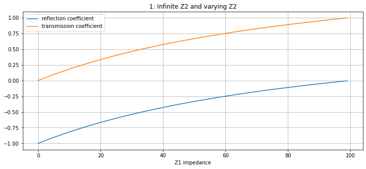
Reflection and transmission coefficients as a function of impedances.

def R_coeff(Z1, Z2):
    return (Z1 - Z2)/(Z1 + Z2)

def P_coeff(Z1, Z2):
    return (2*Z1)/(Z1 + Z2)

Z1 = list(range(0, 100,1))
Z20 = 100 # substitute for infinity but works too

plt.figure(figsize=(12,5))
plt.xlabel("Z1 impedance")

R_coeffs = [R_coeff(item, Z20) for item in Z1]
P_coeffs = [P_coeff(item, Z20) for item in Z1]

plt.plot(Z1, R_coeffs, label = 'reflection coefficient')
plt.plot(Z1, P_coeffs, label = 'transmission coefficient')
plt.legend()
plt.grid(True)
plt.title("1: Infinite Z2 and varying Z2")
plt.show()

plt.figure(figsize=(12,5))
plt.xlabel("Z2 impedance")

Z10 = 10
Z2 = list(range(0, 200,1))

R_coeffs = [R_coeff(Z10, item) for item in Z2]
P_coeffs = [P_coeff(Z10, item) for item in Z2]

x0 = [10]
y0 = [1]
y1 = [0]
plt.plot(x0, y0, "s")
plt.plot(x0, y1, "s")

plt.plot(Z2, R_coeffs, label = 'reflection coefficient')
plt.plot(Z2, P_coeffs, label = 'transmission coefficient')
plt.legend()
plt.grid(True)
plt.title("2: Z1 is a number in between and varying Z2")
plt.show()

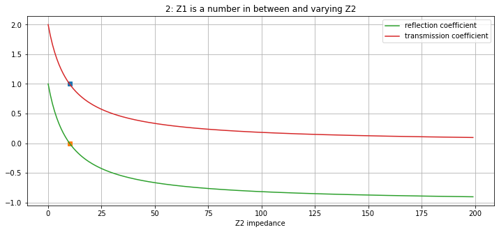
• Note that when \(Z_1 \to 0\) (start of graph 1) and \(Z_2 \to \infty\) (end of graph 2), the reflection coefficient is \(-1\) and transmission coefficient is \(0\). This means that the wave is completely reflected and has a phase change of \(\pi\)

• If \(Z_2\) is zero, the incident wave is reflected, so the reflection coefficient is \(1\), and the transmission coefficient is \(2\). No wave can pass through layer 2 if \(Z_2\) is zero.

• If \(Z_1=Z_2\) (markers on graph 2), the reflection coefficient is \(0\) and the transmission coefficient is \(1\). There is virtually no boundary as the properties, density and seismic velocity, of the media are the same.

Reflection and Transmission (Longitudinal waves)

As longitudinal waves travel through a medium, vibrations lead to pressure waves within the medium, with a phase difference of \(\pi\). Since the longitudinal wave and pressure wave are in anti-phase, the reflection and transmission coefficients for the pressure wave are as follows:

\[ R = \frac{Z_2-Z_1}{Z_1+Z_2} \]

\[ P = \frac{2Z_2}{Z_1+Z_2} \]

References

Imperial College waves lecture notes

https://github.com/geoscixyz/gpgLabs