Chapter 0 – Introduction
Contents
Chapter 0 – Introduction#
Data Science and Machine Learning for Geoscientists
%%javascript
MathJax.Hub.Config({
    TeX: { equationNumbers: { autoNumber: "AMS" } }
});
MathJax.Hub.Queue(
  ["resetEquationNumbers", MathJax.InputJax.TeX],
  ["PreProcess", MathJax.Hub],
  ["Reprocess", MathJax.Hub]
);
There is enough of the introduction about machine learning, so there is no need to elaborate again. This study material helps you understand the codes that classify hand-written digits based on the classic MNIST dataset that can easily be downloaded online (mnist.pkl.gz). Here is how to load the dataset:
"""
mnist_loader
~~~~~~~~~~~~

A library to load the MNIST image data.  For details of the data
structures that are returned, see the doc strings for ``load_data``
and ``load_data_wrapper``.  In practice, ``load_data_wrapper`` is the
function usually called by our neural network code.
"""

#### Libraries
# Standard library
import pickle
import gzip

# Third-party libraries
import numpy as np

def load_data():
    """Return the MNIST data as a tuple containing the training data,
    the validation data, and the test data.

    The ``training_data`` is returned as a tuple with two entries.
    The first entry contains the actual training images.  This is a
    numpy ndarray with 50,000 entries.  Each entry is, in turn, a
    numpy ndarray with 784 values, representing the 28 * 28 = 784
    pixels in a single MNIST image.

    The second entry in the ``training_data`` tuple is a numpy ndarray
    containing 50,000 entries.  Those entries are just the digit
    values (0...9) for the corresponding images contained in the first
    entry of the tuple.

    The ``validation_data`` and ``test_data`` are similar, except
    each contains only 10,000 images.

    This is a nice data format, but for use in neural networks it's
    helpful to modify the format of the ``training_data`` a little.
    That's done in the wrapper function ``load_data_wrapper()``, see
    below.
    """
    f = gzip.open('mnist.pkl.gz', 'rb')
    training_data, validation_data, test_data = pickle.load(f, encoding='latin1')
    f.close()
    return (training_data, validation_data, test_data)

def load_data_wrapper():
    """Return a tuple containing ``(training_data, validation_data,
    test_data)``. Based on ``load_data``, but the format is more
    convenient for use in our implementation of neural networks.

    In particular, ``training_data`` is a list containing 50,000
    2-tuples ``(x, y)``.  ``x`` is a 784-dimensional numpy.ndarray
    containing the input image.  ``y`` is a 10-dimensional
    numpy.ndarray representing the unit vector corresponding to the
    correct digit for ``x``.

    ``validation_data`` and ``test_data`` are lists containing 10,000
    2-tuples ``(x, y)``.  In each case, ``x`` is a 784-dimensional
    numpy.ndarry containing the input image, and ``y`` is the
    corresponding classification, i.e., the digit values (integers)
    corresponding to ``x``.

    Obviously, this means we're using slightly different formats for
    the training data and the validation / test data.  These formats
    turn out to be the most convenient for use in our neural network
    code."""
    tr_d, va_d, te_d = load_data()
    training_inputs = [np.reshape(x, (784, 1)) for x in tr_d[0]]
    training_results = [vectorized_result(y) for y in tr_d[1]]
    training_data = list(zip(training_inputs, training_results))
    validation_inputs = [np.reshape(x, (784, 1)) for x in va_d[0]]
    validation_data = list(zip(validation_inputs, va_d[1]))
    test_inputs = [np.reshape(x, (784, 1)) for x in te_d[0]]
    test_data = list(zip(test_inputs, te_d[1]))
    return (training_data, validation_data, test_data)

def vectorized_result(j):
    """Return a 10-dimensional unit vector with a 1.0 in the jth
    position and zeroes elsewhere.  This is used to convert a digit
    (0...9) into a corresponding desired output from the neural
    network."""
    e = np.zeros((10, 1))
    e[j] = 1.0
    return e
This study material consolidates your understandings by explaining the codes line by line with the maths behind it. The reader is expected to have some basic knowledges about linear algebra and calculus, otherwise we strongly recommend you to go through these materials first (reference a github link here). Note that this material will not cover CNN (Convolutional Neural Network), GAN (Generative Adversarial Network) and RNN (Recurrent Neural Network).
Classification of My Partner’s Decision#
One of the classic exmaple to get you into machine learning is a classfication example. Suppose the weekend is coming up, and my partner has heard that there’s going to be an Imperial open day. She likes Imperial, and is trying to decide whether or not to go to the open day. She might make her decision by weighing up three factors:
Factor |
Condition |
|---|---|
Is the weather good? |
Y/N |
Will I accompany my partner? |
Y/N |
Boris’ Stay Home policy? |
Y/N |
This decision making process is achieved via neural network. To get started, we need to explain a type of artificial neuron called a perceptron. A perceptron takes several binary inputs \(x_1\), \(x_2\), … and produces a single binary output:

In the example shown the perceptron has three inputs, \(x_1\), \(x_2\) and \(x_3\). In general it could have more or fewer inputs. There is a simple rule to compute the output. Here we introduce weights, \(w_1\), \(w_2\), …, real numbers expressing the importance of the respective inputs to the output. The neuron’s output, \(0\) or \(1\), is determined by whether the weighted sum \(\sum_i w_i x_i\) is less than or greater than some threshold value. Just like the weights, the threshold is a real number which is a parameter of the neuron. To put it in more precise algebraic terms:
That’s the basic mathematical model. A way to think about the perceptron is that it’s a device that makes decisions by weighing up evidence. For instance, we’d have \(x_1=1\) if the weather is good, and \(x_1=0\) if the weather is bad. Similarly, \(x_2=1\) if I want to accompany my partner, and \(x_2=0\) if not. And similarly again for \(x_3\) and stay home policy.
Now, suppose my partner absolutely adores Imperial, so much so that she/he is happy to go to the open day even if I was uninterested and the Boris said “Please stay at home and save lives” many many times. Or perhaps she/he really loathes bad weather, and there’s no way she’d go to the open day if the weather is bad. We can use perceptrons to model this kind of decision-making. One way to do this is to choose a weight \(w_1=6\) for the weather, and \(w_2=2\) and \(w_3=2\) for the other conditions. The larger value of \(w_1\) indicates that the weather matters a lot to my partner, much more than whether I join or the stay home policy. Finally, suppose we choose a threshold of 5 for the perceptron. With these choices, the perceptron implements the desired decision-making model, outputting 1 whenever the weather is good, and 0 whenever the weather is bad. It makes no difference to the output whether I want to join my partner, or whether Boris’ spank those who do not stay at homes.
By varying the weights and the threshold, we can get different models of decision-making. For example, suppose we instead chose a threshold of 3. Then the perceptron would decide that my partner should go to the festival whenever the weather was good or when both the stay home policy is lifted and I want to join her/him. In other words, it’d be a different model of decision-making. Dropping the threshold means she/he is more willing to go to the festival under the same 3 circumstances.
The key, however, is to find the weights \(w\) and bias \(b\) term in her/his mind as we do not know them in advanced. Maybe she/he hates me so \(w_2 = 0\) or maybe she/he is really picky \(b = 100\). We don’t know. But that’s the whole point of machine learning, to know those values to some extent.
Classification of Admission Data#
Here is another example to get you into the world of Machine Learning. Suppose the university admission is dependent on two factors: \(\boldsymbol SAT\) and \(\boldsymbol GPA\) scores. Then we can have a list of students with their application details who applied to one of the best universities in the universe, the University of Jianou.
SAT |
GPA |
Offer? |
|---|---|---|
800 |
3.95 |
Y |
710 |
2.7 |
N |
750 |
3.4 |
N |
690 |
3.82 |
Y |
600 |
4.00 |
N |
… |
… |
… |
The University of Jianou is founded at the end of 2019 so the admission data in 2020 can be regarded as the norm of all the admission data. We want to build a model, based on the 2020 data, to predict if Barron Trump can make it into Jianou University with his scores.
SAT |
GPA |
Offer? |
|---|---|---|
530 |
1.6 |
? |
For human beings, it is fairly easy to have a sense of feeling of whether this kid can make it into the top university with such low grades. However, this sense of feeling is extremely hard for computer to understand. Our aim is to train the computer model to have this sense of feeling (potentially better than us) to make predictions.
Mathematically, we can express SAT, GPA and offer result as \(x_1\), \(x_2\) and \(y\). \(y\) is binary as in it is \(0\) when \(y=N\) and \(1\) when \(y=Y\). In a sense, we can have the following table that is a quantified version of the admission data.
\(x_1\) |
\(x_2\) |
y |
|---|---|---|
800 |
3.95 |
1 |
710 |
2.7 |
0 |
750 |
3.4 |
0 |
690 |
3.82 |
1 |
600 |
4.00 |
0 |
… |
… |
… |
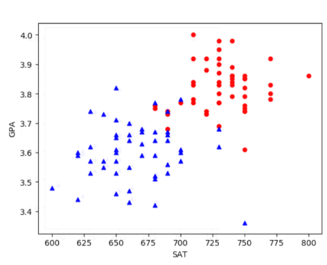 Figure 1.1: Visualisation of SAT and GPA; the red dot representsyvalue being Y and bluetriangle meansyvalue being N.
We realise that the students with higher GPA and higher SAT grades are more likely to be accepted, or the group of red dots in the upper right corner. In contrast, the students in the lower left are all rejected. There seems to be a line that separates the two groups. We can express the equation of such line as
where \(w_1\) and \(w_2\) are weights, meaning how important their corresponding \(x\)s are; the bigger the \(w_1\) the more important SAT in the admission process and vice versa.
The trick is to find the \(w_1\) and \(w_2\) that best separates the two groups.
Based on Figure 1.1, we know that Barron Trump will receive an offer if
and will not receive an offer if
This is such a common used equation, so we can give it a general form
To summarize his admission result, we can have the following equation (which is the same as equation (1)).