Recursion#

Recursion is a method of solving Computer Science problems by considering smaller instances of the same problem. Recursive solutions are usually implemented with functions that call themselves. Consider the example of the factorial function:

def fact(n):
    assert n >=0

    if n == 0:
        return 1
    elif n == 1:
        return 1
    else:
        return n*fact(n-1)
          
print(fact(1))
print(fact(5))

1
120

Usually, a recursively defined function has two basic building blocks:

Base case (cases): Which are used for specific (finite) subsets of possible inputs. In the example, this will be when \(n=0\) or \(n=1\). In these cases, the function should not refer to itself.
Recursive case (cases): This case builds on the smaller version of the same problem. In this case, we are decrementing the value of \(n\) before calling the function again.

The broad idea that recursive cases should assure that the function reaches one of the base cases.

Famous examples#

Greatest common divisor Probably the most well known recursive algorithm developed by Euclid:

def gcd(a,b):
    if b == 0:#base case
        return a
    else: #recursive case
        return gcd(b,a%b)
        
print(gcd(1,9))
print(gcd(15,12))

1
3

Fibonacci Sequence To compute the \(n\)-th term of the Fibonacci, we can utilise one of its definitions as in the code below:

def fib(n):
    assert n >=0
    
    if n == 0: #Base case
        return 1
    elif n == 1: #Base case
        return 1
    else: #Inductive case
        return fib(n-2)+fib(n-1)
    
    
print(fib(1))
print(fib(10))

1
89

REMARK: This is a very inefficient solution. As you can spot, each fib call leads to two fib calls (unless it reaches a base case). This solution is of \(O(2^n)\), which is very slow. We can use Dynamic Programming to speed it up.

Towers of Hanoi In this problem, we have three rods and some disks of different sizes. Our aim is to move all disks from one rod to another using the third rod. The following rules apply:

Only one disk can be moved at a time.
Each move consists of taking the upper disk from one of the stacks and placing in on the other.
No larger disk may be placed on top of a smaller disk.

Source: Wikimedia Commons

The solution is likely one of the most beautiful recursive procedures:

We are starting with \(n\) disks on the source rod and want to move them to the target rod, with the help of the spare rod. The procedure is as follows:

Base Case:

There are zero disks, do nothing.

Recursive case:

Move \(n-1\) disks from the source the the spare by the main solving procedure. This leaves disk \(n\) on top of the source rod.
Move the \(n\) disk from the source to the target.
Move \(n-1\) disks from spare to the source by the main solving procedure.

The code is as follows:

def hanoi(n, source, target,spare):
    assert n >= 0
    if n > 0: 
        
        #(1)
        hanoi(n-1,source, spare, target)
        #(2)
        target.append(source.pop())
        
        print(A, B, C, '______________', sep='\n')
        #(3)
        hanoi(n-1,spare,target,source)
    
A = [4,3, 2, 1]
B = []
C = []

hanoi(4, A, C, B)

[4, 3, 2]
[1]
[]
______________
[4, 3]
[1]
[2]
______________
[4, 3]
[]
[2, 1]
______________
[4]
[3]
[2, 1]
______________
[4, 1]
[3]
[2]
______________
[4, 1]
[3, 2]
[]
______________
[4]
[3, 2, 1]
[]
______________
[]
[3, 2, 1]
[4]
______________
[]
[3, 2]
[4, 1]
______________
[2]
[3]
[4, 1]
______________
[2, 1]
[3]
[4]
______________
[2, 1]
[]
[4, 3]
______________
[2]
[1]
[4, 3]
______________
[]
[1]
[4, 3, 2]
______________
[]
[]
[4, 3, 2, 1]
______________

Recursive Data Structures#

Apart from the algorithms themselves, we can structure (or interpret) our data in a recursive way. Any time we can reduce an instance of the data structure to the same but somehow smaller, we can talk about a recursively defined data structures. It turns out that many structures can be defined this way:

Lists can be thought of as a single element (head) followed by a tail (again a list). The base case is an empty list.

import copy
class RecList:
    def __init__(self):
        self.head = None
        self.tail = None
        
    def add(self,elem):
        self.tail = copy.deepcopy(self)
        self.head = elem
        
    def __str__(self):
        if self.tail is None:
            return "[]"
            
        else:
            return "(" + str(self.head) + ":" + str(self.tail) + ")"
        
        
l = RecList()
l.add(1)
l.add(2)
l.add(3)
print(l)

(3:(2:(1:[])))

Where the copy.deepcopy returns a copy of the list. When defined this way, the list consists of a leading element and a list one-smaller than the parent list.

We can now use this definition to sum up the elements of an integer list (with standard Python list implementation):

def array_sum(x):
    if x == []:
        return 0
    else:
        return x[0] + array_sum(x[1:])
    
array_sum([1,2,3,4,5,6,7,8,9])

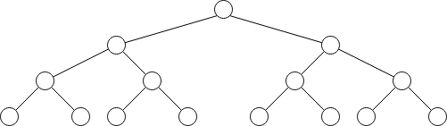
Binary Trees are types of graphs that do not have cycles and each node has at most two children and exactly one parent. They are self-similar as both of the subtrees of such binary tree are also trees. This is a characteristic feature of recursive data structures.

Exercises#

Length of an array Based on the array_sum function, define a recursive function which counts the number of elements in an array.

Answer

def array_len(a):
    if a == []:
        return 0
    else:
        return 1 + array_len(a[1:])     

Babylonian Square Roots A method to find an approximation of a square root of a number \(S\) is to pick a guess \(x_0\) and iteratively improve the guess by applying the formula \(x_1 = (x_0 + S/x_0)\). In the limit, this will give a square root. Unfortunately, we do not have time for an infinite number of operations, so return \(x_1\) when the condition is satisfied:

\[\frac{|x_1-x_0|}{x_1} < 0.01\]

Answer

def babSqrtHelper(S, x_0, x_1):
    if abs(x_1-x_0)/x_1 < 0.01:
        return x_1
    else:
        return babSqrtHelper(S,x_1,(x_1+S/x_1)/2)

def babSqrt(S):
    x_0 = S
    x_1 = (x_0 + S/x_0)/2
    return babSqrtHelper(S, x_0, x_1)

print(babSqrt(1))
print(babSqrt(2))
print(babSqrt(3))
print(babSqrt(4))    

Design a BinaryTree data structure. Each node should have a left and right child fields as well as a value inside the node. Define also two other methods:

Insert: inserts value into the tree if the element is greater than its parent it goes to the right subtree if smaller - to the left one. Finally, if the element is already in the tree, do not add it and inform the user about it.
Search: search if the element is in the list.

Answer

class BinaryTree:
    def __init__(self):
        self.left = None
        self.right = None
        self.val = None

    def insert(self,val):
        if self.val is None:
            self.val = val
        elif self.val == val:
            print("Value already in the tree!")
        elif self.val < val:
            if self.right is None:
                self.right = BinaryTree()
            self.right.insert(val)
        else:
            if self.left is None:
                self.left = BinaryTree()
            self.left.insert(val)


    def search(self,val):
        if self.val is None:
            return False
        elif self.val < val:
            if self.right is None:
                return False
            return self.right.search(val)
        elif self.val > val:
            if self.left is None:
                return False
            return self.left.search(val)
        else:
            return True
            
        
root = BinaryTree()
root.insert(1)
root.insert(2)  
root.insert(3) 
print(root.search(1))  
print(root.search(0))   
             

References#

Sebastian Raschka, GitHub, Algorithms in IPython Notebooks
Cormen, Leiserson, Rivest, Stein, “Introduction to Algorithms”, Third Edition, MIT Press, 2009

ESE Jupyter Material

Recursion

Contents

Recursion#

Famous examples#

Recursive Data Structures#

Exercises#

References#