Google Earth Engine foundations#

Advanced Remote Sensing

This notebooks aims to walk you through and clarify some of the basic concept of using the Google Earth engine by building upon our script step by step. Majority of this content has been borrowed from this github repository containing over 360+ Jupyter Python notebooks examples to demonstrate the Google Earth Engine guide in python notebooks.

Setting up your notebook#

# Installs geemap package
import subprocess

try:
    import geemap
except ImportError:
    print('geemap package not installed. Installing ...')
    subprocess.check_call(["python", '-m', 'pip', 'install', 'geemap'])

# Checks whether this notebook is running on Google Colab
try:
    import google.colab
    import geemap.eefolium as geemap
except:
    import geemap

# Authenticates and initializes Earth Engine
import ee

try:
    ee.Initialize()
except Exception as e:
    ee.Authenticate()
    ee.Initialize()

#set map
Map = geemap.Map(center=[40,-100], zoom=4)
#Set a basemap, standard is google maps
Map.add_basemap('SATELLITE')
Map

Display an image#

# Load an image.
image = ee.Image('LANDSAT/LC08/C01/T1/LC08_044034_20140318')

# Display the image.
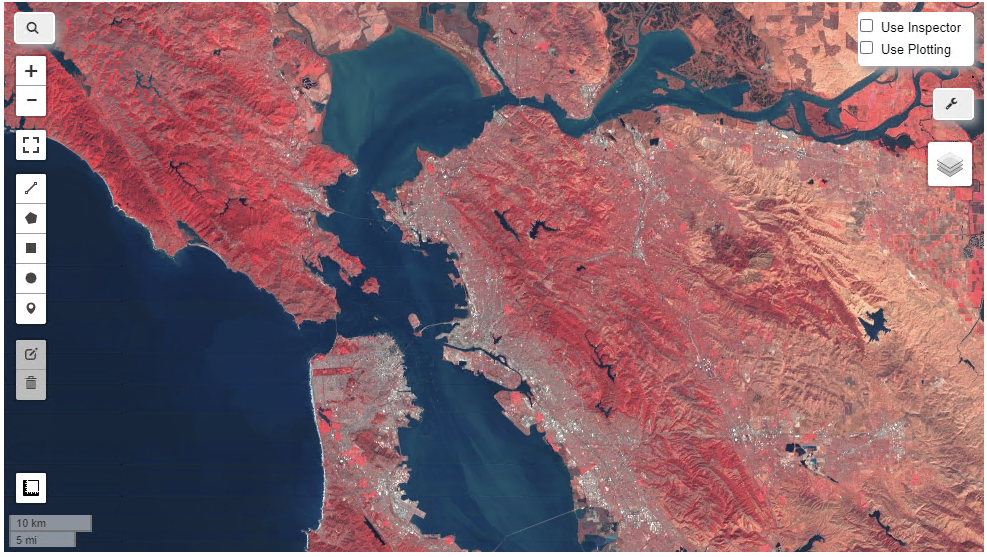
Map.addLayer(image, {}, 'Landsat 8 original image')
Map.centerObject(image, 7)
#show Map
Map

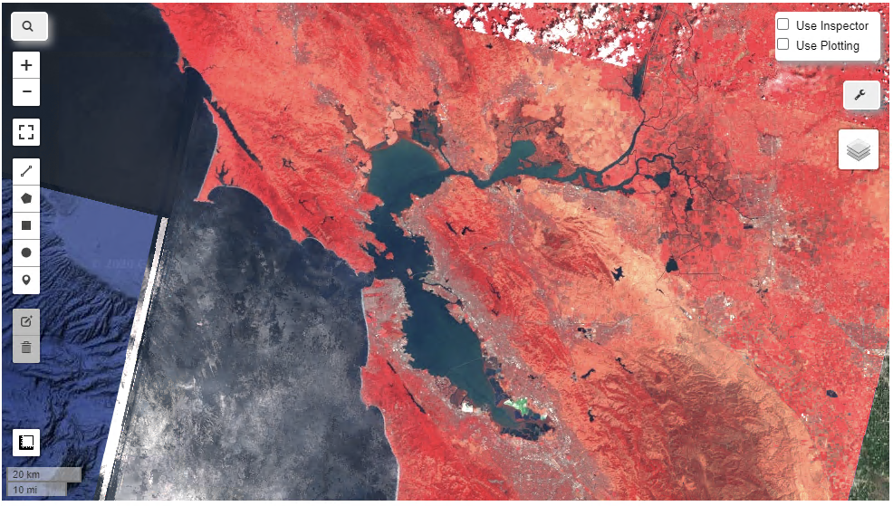
Visualise specific bands#

Remember multiple bands are displayed as RGB to our eyes.

# Define visualization parameters in an object literal.
vizParams = {'bands': ['B5', 'B4', 'B3'],
            'min': 5000, 'max': 15000, 'gamma': 1.3}

# Center the map on the image and display.
Map.centerObject(image, 7)
Map.addLayer(image, vizParams, 'Landsat 8 False color')
Map

Find an image#

it is highly recommended to first look at the Google Earth Engine database before starting to filter for an image in your script. Each dataset on the website also has a few lines of code showing how to access it.

#set location, easy to find on google maps
point = ee.Geometry.Point(-122.262, 37.8719)

#set filter criteria
filteredCollection = ee.ImageCollection('LANDSAT/LC08/C01/T1') \
    .filterBounds(point) \
    .filterDate('2014-06-01','2014-10-01') \
    .sort('CLOUD_COVER', True)   #sort by cloudcover

#see how many images in collection
print(filteredCollection.size().getInfo())

#take 1st image from collection, least cloudy one
first = filteredCollection.first()

# Define visualization parameters in an object literal.
vizParams = {'bands': ['B5', 'B4', 'B3'],
             'min': 5000, 'max': 15000, 'gamma': 1.3}

# Center the map on the image and display.
Map.centerObject(point, 9)
Map.addLayer(first, vizParams, 'Landsat 8 image')
Map

Band maths#

There are many more functions than the below which can be applied, they are found in the linked manuals. but here is a demonstration on how they work.

# find image
point = ee.Geometry.Point(-122.262, 37.8719)

filteredCollection = ee.ImageCollection('LANDSAT/LC08/C01/T1') \
    .filterBounds(point) \
    .filterDate('2014-06-01','2014-10-01') \
    .sort('CLOUD_COVER', True)   #sort by cloudcover

#take 1st image from collection, least cloudy one
first = filteredCollection.first()

#define function to be applied to image
def getNDWI(image):    # (B5 - B3)/(B5+B3)
    return image.normalizedDifference(['B5', 'B3'])
#apply function to image
ndwi1 = getNDWI(first)

# Define visualization parameters in an object literal.
ndwiParams = {'min': -0.5, 'max': 0.5, 'palette': ['FF0000', 'FFFFFF', '0000FF']}

# Center the map on the image and display.
Map.centerObject(point, 9)
Map.addLayer(ndwi1, ndwiParams, 'NDVI 1')
Map

Apply band math to an image collection#

# Add Earth Engine dataset
point = ee.Geometry.Point(-122.262, 37.8719)

filteredCollection = ee.ImageCollection('LANDSAT/LC08/C01/T1') \
    .filterBounds(point) \
    .filterDate('2014-06-01','2014-10-01') \
    .sort('CLOUD_COVER', True)   #sort by cloudcover

#visualise bands available for images in collection
#Landsat 8 expected 11 bands
bandNames = filteredCollection.first().bandNames()
print(bandNames.getInfo())

#carry out function and add output as an extra band
def addNDVI(image):
    return image.addBands(image.normalizedDifference(['B5', 'B3']))

# Map the function over the collection.
ndviCollection = filteredCollection.map(addNDVI)
# you can see we created a new band containing our function above
first = ndviCollection.first()
bandNames = first.bandNames()
print(bandNames.getInfo())

Reducing#

Reducing enhances common information between images and reduces noise like cloud cover by averaging multiple images.

# Add Earth Engine dataset
collection = ee.ImageCollection('LANDSAT/LC08/C01/T1') \
    .filterBounds(ee.Geometry.Point(-122.262, 37.8719)) \
    .filterDate('2014-01-01', '2014-12-31') \
    .sort('CLOUD_COVER')

# Compute the median of each pixel for each band of the 5 least cloudy scenes.
median = collection.limit(5).reduce(ee.Reducer.median())

# Define visualization parameters in an object literal.
vizParams = {'bands': ['B5_median', 'B4_median', 'B3_median'],
             'min': 5000, 'max': 15000, 'gamma': 1.3}
# display image
Map.setCenter(-122.262, 37.8719, 10)
Map.addLayer(median, vizParams, 'Median image')
Map

Obtain image statistics#

# Add Earth Engine dataset
image = ee.Image('LANDSAT/LC08/C01/T1_TOA/LC08_044034_20140318')
Map.addLayer(image, {'bands': ['B4', 'B3', 'B2'], 'max': 0.3}, 'Landsat 8')

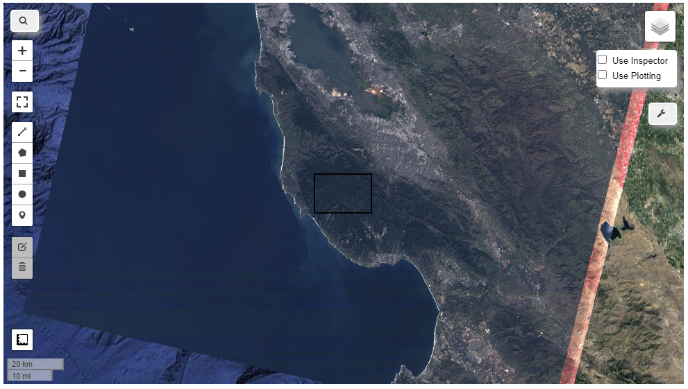
# Create an arbitrary rectangle as a region and display it.
region = ee.Geometry.Rectangle(-122.2806, 37.1209, -122.0554, 37.2413)
Map.centerObject(ee.FeatureCollection(region), 9)
Map.addLayer(ee.Image().paint(region, 0, 2), {}, 'Region')

# Get a dictionary of means in the region. Keys are bandnames.
mean = image.reduceRegion(**{
  'reducer': ee.Reducer.mean(),
  'geometry': region,
  'scale': 30
})

print(mean.getInfo())
Map

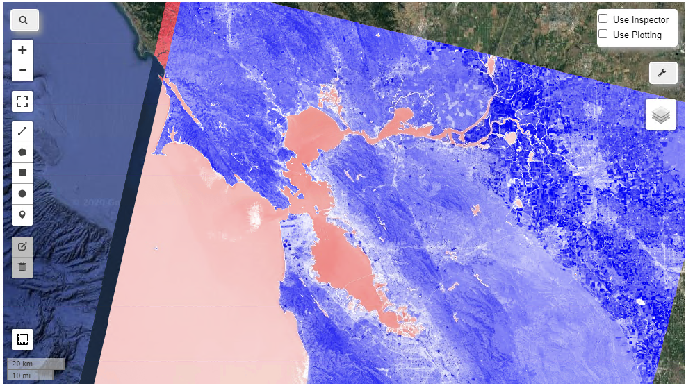
Using masks#

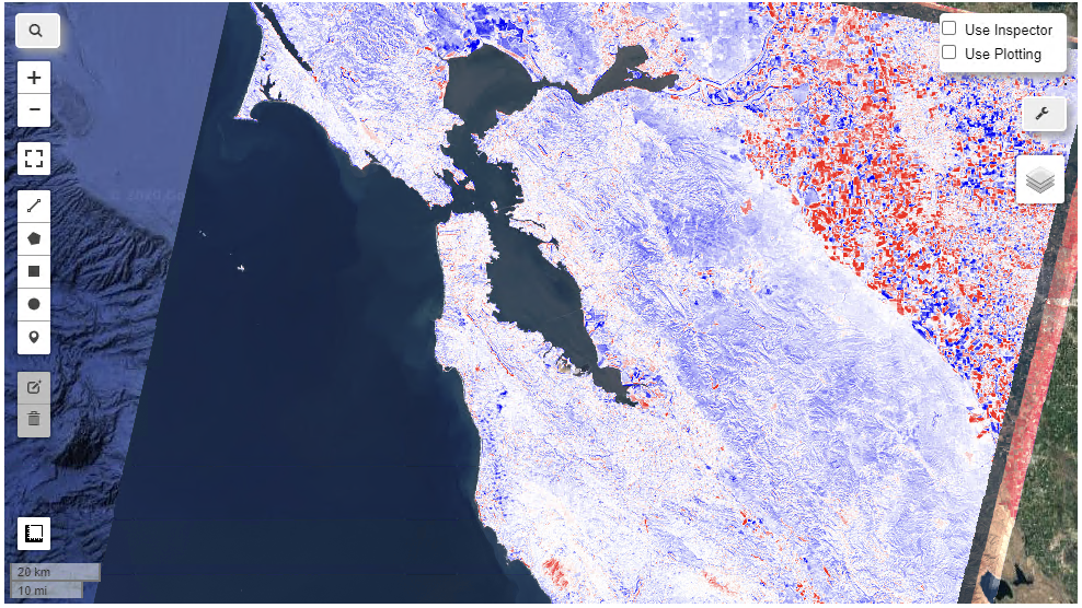
The mask in the example below avoids us from including the water bodies in our data, this way we have a wider range of our colour palette available to show changes on land.

# Load two Landsat 5 images, 20 years apart.
image1 = ee.Image('LANDSAT/LT05/C01/T1_TOA/LT05_044034_19900604')
image2 = ee.Image('LANDSAT/LT05/C01/T1_TOA/LT05_044034_20100611')


# This function gets NDVI from Landsat 5 imagery.
def getNDVI(image):
    return image.normalizedDifference(['B4', 'B3'])

# Compute NDVI from the scenes.
ndvi1 = getNDVI(image1)
ndvi2 = getNDVI(image2)

# Compute the difference in NDVI.
ndviDifference = ndvi2.subtract(ndvi1)

# Load the land mask from the SRTM DEM.
landMask = ee.Image('CGIAR/SRTM90_V4').mask()

# Update the NDVI difference mask with the mask
maskedDifference = ndviDifference.updateMask(landMask)

# Display the masked result.
vizParams = {'min': -0.5, 'max': 0.5,
             'palette': ['FF0000', 'FFFFFF', '0000FF']}
Map.setCenter(-122.2531, 37.6295, 9)
Map.addLayer(maskedDifference, vizParams, 'NDVI difference')
Map

Inbuild CloudScore function#

## mask clouds
def cloudMask(img):
    cloudscore = ee.Algorithms.Landsat.simpleCloudScore(img).select('cloud')
    return img.updateMask(cloudscore.lt(50))

# Add Earth Engine dataset
collection = ee.ImageCollection('LANDSAT/LC8_L1T_TOA') \
                .filterDate('2014-12-10', '2016-12-31') \
                .filterBounds(ee.Geometry.Point(-122.262, 37.8719)) \
                .map(cloudMask) #hash in front to see difference

print(collection.size().getInfo())

#average images in collection
median = collection.median()
#display image
Map.setCenter(-122.262, 37.8719, 9)
vis = {'bands': ['B5', 'B4', 'B3'], 'max': 0.3}
Map.addLayer(median,vis)
Map

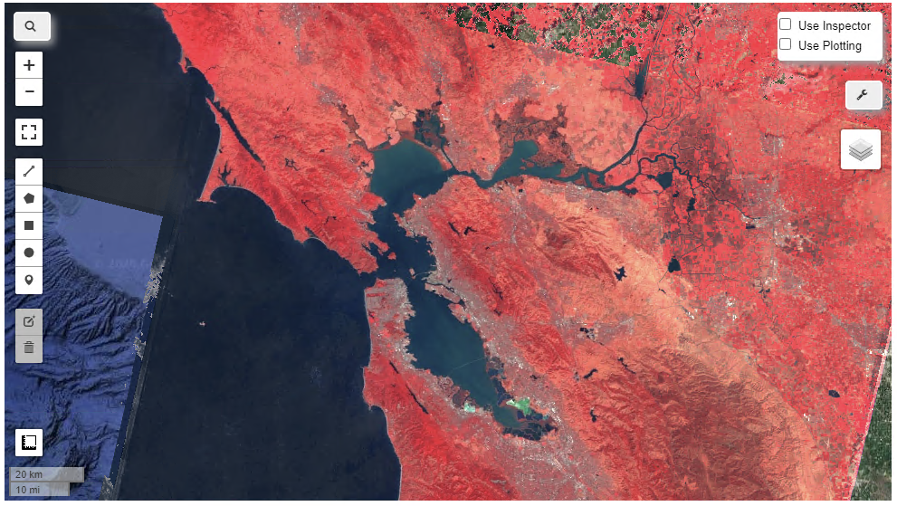
With CloudMask function: Without CloudMask function:

ESE Jupyter Material

Google Earth Engine foundations

Contents