Rate Law
Contents
Rate Law#
Chemistry for Geoscientists Low-Temperature Geochemistry
Rate law is an expression of the empirical dependence of the rate of reaction on the concentrations of the reactants.
Consider the following chemical equation:
So, the rate (\(R\)) of the reaction can be written as:
where
\(k\) = experimentally determined rate constant (sometimes also called “specific rate constant”)
\(n_A\), \(n_B\), … are real numbers (can be fractions, or zero) that denote the “order of the reaction” with respect to species A, B, C, D,…
\(n_{overall}=n_A+n_B+...\) is the overall order of the reaction
“order \(n_i\)” not typically the same as stoichiometry (\(v_i\)) BUT IT CAN BE for elementary reactions, if mechanism is known (number of individual atoms/molecules involved in the reaction)
To make everything simple, we will conider reactions with only one reactant, but different orders.
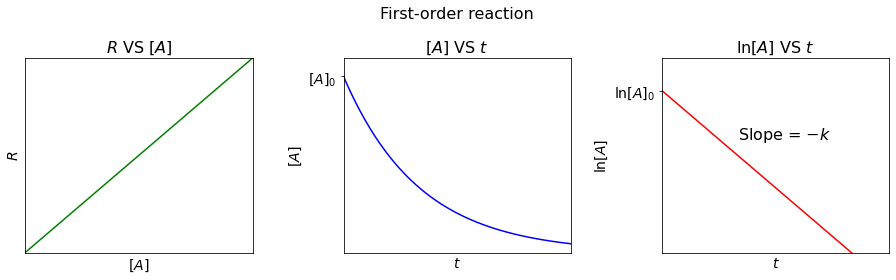
First-order reaction#
For a first-order reaction, the reaction rate (\(R\)) is directly proportional to the concentration of the reactant, i.e.
Rearranging the rate law, we get
Integrating it, we get
So, we can plot a linear relationship between \(\ln[A]\) and \(t\), with slope = \(-k\) and y-intercept = \(\ln[A]_0\).
Finding t when \([A]=\frac{[A]_0}{2}\).
The time the concentration of a reactant takes to reach half it’s starting value is called “half-life (\(t_{\frac{1}{2}}\))”. It can be seen that, for first-order reactions, the length of half-life is independent of the concentration of a reactant.
# import relevant modules

%matplotlib inline
from math import e
import numpy as np
import matplotlib.pyplot as plt
import pandas as pd
from IPython.display import display
# create our own functions

def dont_show_scale(ax, axis):
    if axis == 'x':
        ax.set_xticks([])
        ax.set_xticklabels([])
    elif axis == 'y':
        ax.set_yticks([])
        ax.set_yticklabels([])
    return ax

def simple_title_and_label(ax, x_name, y_name):
    ax.set_title(y_name + ' VS ' + x_name, fontsize=16)
    ax.set_xlabel(x_name, fontsize=14)
    ax.set_ylabel(y_name, fontsize=14)
    return ax

# define a function to mimic the empirical rate law (rate = k[A]^n)
def rate(A, k, n):
    return k*(A**n)
# set figures
fig, (ax1, ax2, ax3) = plt.subplots(1, 3, figsize=(10, 4))
fig.suptitle("First-order reaction", fontsize=16)
plt.subplots_adjust(top=0.8,
                    left=-0.1,
                    right=1.1,
                    wspace=0.4,
                    hspace=0.4)

k = 1  # rate constant
A0 = e  # [A]0

# define functions to mimic the integrated rate law
def integrated_A_1st_order(t, k, A0):
    return A0*(e**(-k*t))

def integrated_lnA_1st_order(t, k, A0):
    return np.log(integrated_A_1st_order(t, k, A0))

# plot Rate VS [A]
A = np.linspace(0, 1.2, 100)
ax1.plot(A, rate(A, k, 1), 'g')
ax1.set_xlim(0, 1.2)
ax1.set_ylim(0, 1.2)
simple_title_and_label(ax1, '$[A]$', '$R$')
dont_show_scale(ax1, 'x')
dont_show_scale(ax1, 'y')

# plot [A] VS t
t = np.linspace(0, 3, 100)
ax2.plot(t, integrated_A_1st_order(t, k, A0), 'b')
ax2.set_xlim(0, 3)
ax2.set_ylim(0, 3)
simple_title_and_label(ax2, '$t$', '$[A]$')
dont_show_scale(ax2, 'x')
ax2.set_yticks([A0])
ax2.set_yticklabels(['$[A]_0$'], fontsize=14)

# plot ln[A] VS t
t = np.linspace(0, 1.2, 100)
ax3.plot(t, integrated_lnA_1st_order(t, k, A0), 'r')
ax3.set_xlim(0, 1.2)
ax3.set_ylim(0, 1.2)
simple_title_and_label(ax3, '$t$', '$\ln[A]$')
dont_show_scale(ax3, 'x')
ax3.set_yticks([integrated_lnA_1st_order(0, k, A0)])
ax3.set_yticklabels(['$\ln[A]_0$'], fontsize=14)
ax3.text(0.4, 0.7, 'Slope = $-k$', fontsize=16)
Text(0.4, 0.7, 'Slope = $-k$')
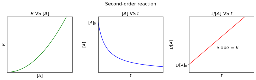
Second-order reaction#
For a second-order reaction, the reaction rate (\(R\)) is directly proportional to the square of the concentration of the reactant, i.e.
Derived by the similar approach, the integrated rate law can be written as:
So, we can plot a linear relationship between \(\frac{1}{[A]}\) and \(t\), with slope = \(k\) and y-intercept = \(\frac{1}{[A]_0}\).
And half-life (\(t_{\frac{1}{2}}\)) is:
Contrast to first-order reactions, the half-life of a second-order reaction is dependent on the concentration of a reactant.
# set figures
fig, (ax1, ax2, ax3) = plt.subplots(1, 3, figsize=(10, 4))
fig.suptitle("Second-order reaction", fontsize=16)
plt.subplots_adjust(top=0.8,
                    left=-0.1,
                    right=1.1,
                    wspace=0.4,
                    hspace=0.4)

k = 1  # rate constant
A0 = e  # [A]0

# define functions to mimic the integrated rate law
def integrated_1_over_A_2nd_order(t, k, A0):
    return (1/A0)+k*t

def integrated_A_2nd_order(t, k, A0):
    return 1/integrated_1_over_A_2nd_order(t, k, A0)

# plot Rate VS [A]
A = np.linspace(0, 1.2, 100)
ax1.plot(A, rate(A, k, 2), 'g')
ax1.set_xlim(0, 1.2)
ax1.set_ylim(0, 1.2)
simple_title_and_label(ax1, '$[A]$', '$R$')
dont_show_scale(ax1, 'x')
dont_show_scale(ax1, 'y')

# plot [A] VS t
t = np.linspace(0, 3, 100)
ax2.plot(t, integrated_A_2nd_order(t, k, A0), 'b')
ax2.set_xlim(0, 3)
ax2.set_ylim(0, 3)
simple_title_and_label(ax2, '$t$', '$[A]$')
dont_show_scale(ax2, 'x')
ax2.set_yticks([A0])
ax2.set_yticklabels(['$[A]_0$'], fontsize=14)

# plot 1/[A] VS t
t = np.linspace(0, 1.2, 100)
ax3.plot(t, integrated_1_over_A_2nd_order(t, k, A0), 'r')
ax3.set_xlim(0, 1.2)
ax3.set_ylim(0.2, 1.4)
simple_title_and_label(ax3, '$t$', '$1/[A]$')
dont_show_scale(ax3, 'x')
ax3.set_yticks([integrated_1_over_A_2nd_order(0, k, A0)])
ax3.set_yticklabels(['$1/[A]_0$'], fontsize=14)
ax3.text(0.5, 0.7, 'Slope = $k$', fontsize=16)
Text(0.5, 0.7, 'Slope = $k$')
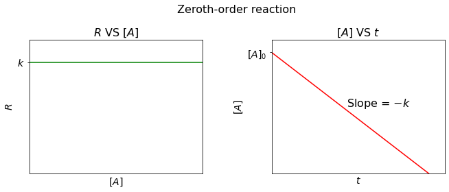
Zeroth-order reaction#
For a zeroth-order reaction, the reaction rate (\(R\)) is constant over time, regardless of the concentration of reactants, i.e.
Derived by the similar approach, the integrated rate law can be written as:
So, we can plot a linear relationship between \([A]\) and \(t\), with slope = \(-k\) and y-intercept = \([A]_0\).
And half-life (\(t_{\frac{1}{2}}\)) is:
# set figures
fig, (ax1, ax2) = plt.subplots(1, 2, figsize=(7, 4))
fig.suptitle("Zeroth-order reaction", fontsize=16)
plt.subplots_adjust(top=0.8,
                    left=-0.1,
                    right=1.1,
                    wspace=0.4,
                    hspace=0.4)

k = 1  # rate constant
A0 = e  # [A]0

# define a function to mimic the integrated rate law
def integrated_A_0th_order(t, k, A0):
    return A0-k*t

# plot Rate VS [A]
A = np.linspace(0, 1.2, 100)
ax1.plot(A, rate(A, k, 0), 'g')
ax1.set_xlim(0, 1.2)
ax1.set_ylim(0, 1.2)
simple_title_and_label(ax1, '$[A]$', '$R$')
dont_show_scale(ax1, 'x')
ax1.set_yticks([rate(0, k, 0)])
ax1.set_yticklabels(['$k$'], fontsize=14)

# plot [A] VS t
t = np.linspace(0, 3, 100)
ax2.plot(t, integrated_A_0th_order(t, k, A0), 'r')
ax2.set_xlim(0, 3)
ax2.set_ylim(0, 3)
simple_title_and_label(ax2, '$t$', '$[A]$')
dont_show_scale(ax2, 'x')
ax2.set_yticks([A0])
ax2.set_yticklabels(['$[A]_0$'], fontsize=14)
ax2.text(1.3, 1.5, 'Slope = $-k$', fontsize=16)
Text(1.3, 1.5, 'Slope = $-k$')
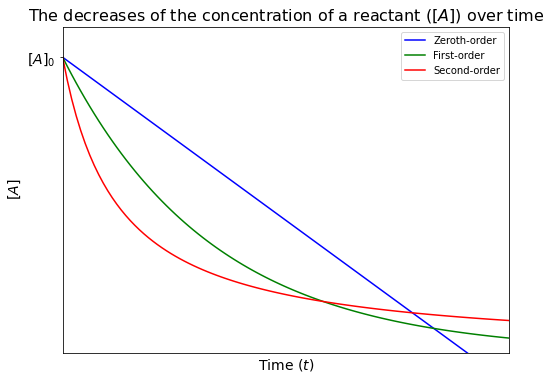
The plot below is created to compare the decrease of the concentration of a reactant over time for reactions with different orders.
k = 1  # rate constant
A0 = e  # [A]0

# plot [A] VS t
plt.figure(figsize=(8,6))
t = np.linspace(0, 3, 100)
plt.plot(t, integrated_A_0th_order(t, k, A0), 'b', label='Zeroth-order')
plt.plot(t, integrated_A_1st_order(t, k, A0), 'g', label='First-order')
plt.plot(t, integrated_A_2nd_order(t, k, A0), 'r', label='Second-order')
plt.xlim([0, 3])
plt.ylim([0, 3])
plt.xticks([], [])
plt.yticks([A0], ['$[A]_0$'], fontsize=14)
plt.xlabel('Time $(t)$', fontsize=14)
plt.ylabel('$[A]$', fontsize=14)
plt.title('The decreases of the concentration of a reactant ($[A]$) over time', fontsize=16)
plt.legend(loc='best', fontsize=10)
<matplotlib.legend.Legend at 0x22e8ae570d0>
Lesson 6 - Problem 1#
Use an empirical rate law to calculate the influence of \(pH\) on reaction rate. (from N. Eby, example 2-7, p44)
At \(pH>4\), the oxidation of \(Fe^{2+}\) in solution can be expressed by the following net reaction
It turns out that the empirical rate law for the reaction is given by
\(k_+\) is the rate constant for the forward reaction. At \(20^\circ C\), it is measured to be
The partial pressure of oxygen in the atmosphere is about \(P_{O_2}=0.2\,bar\).
Assuming that the concentration of \([Fe^{2+}]\) is measured and equals \(10^{-3}\,mol\,L^{-1}\), calculate the reaction rate of the oxidation of \([Fe^{2+}]\) at \(pH=5\) and \(pH=7\).
At \(pH=5\), \([H^+]=10^{-5}\,M\)
At \(pH=7\), \([H^+]=10^{-7}\,M\)
We can find the relationship between \(pH\) and the reaction rate as both are related to \([H^+]\) as follows.
Recall the given empirical rate law:
Gathering all the constants, we get:
where \(K = k_+[Fe^{2+}]\cdot P_{O_2}\) is a constant.
Since \(pH = -\log[H^+]\), so:
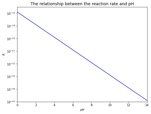
From the relationship, it can be seen that increasing \(pH\) for this reaction can affect the rate by orders of magnitude, as depicted in the plot below. Note that the negative sign, which means that \([Fe(II)]\) experiences a decrease, will be omitted.
# Calculate the value of K
K = (1.2*10**-11) * (10**-3) * 0.2

# plot
plt.figure(figsize=(8,6))
pH = np.linspace(0, 14, 100)
plt.plot(pH, K/(10**(2*pH)), 'b')
plt.xlabel('$pH$')
plt.ylabel('$R$')
plt.xlim([0, 14])
plt.ylim([10**-43, 10**-13])
plt.yscale("log")
plt.title('The relationship between the reaction rate and pH', fontsize=14)
Text(0.5, 1.0, 'The relationship between the reaction rate and pH')
References#
Lecture slide and practical for Lecture 6 of the Low-Temperature Geochemistry module