Graph Algorithms
Contents
Graph Algorithms#
Graph#
In broad terms. A graph \((V,E)\) is an abstract structure consisting of nodes (vertices) and edges connecting some of them. Graphs can be directed or undirected which means that their edges can be traversed in one or both directions. Graphs can be unweighted or not, their edges can have assigned weights. There are several ways of representing graphs in computers, two of which are:
Adjecency matrix \(A\): Which are matrices consisting of \(1\) and \(0\). A \(1\) at a coordinates \((i,j)\) means that there is an edge from node \(i\) to node \(j\). For undirected graphs \(A[i,j]\) = \(A[j,i]\). Adjacency matricex are a compact way of representing dense graphs where the number of edges is close to \(|V|^2\).
Adjacency list \(L\): which is a 2D array where an entry \(L[i]\) is a list with the ids of nodes to which \(i\) is connected to. It is a space-efficient representation for sparse graphs where not many nodes are connected.
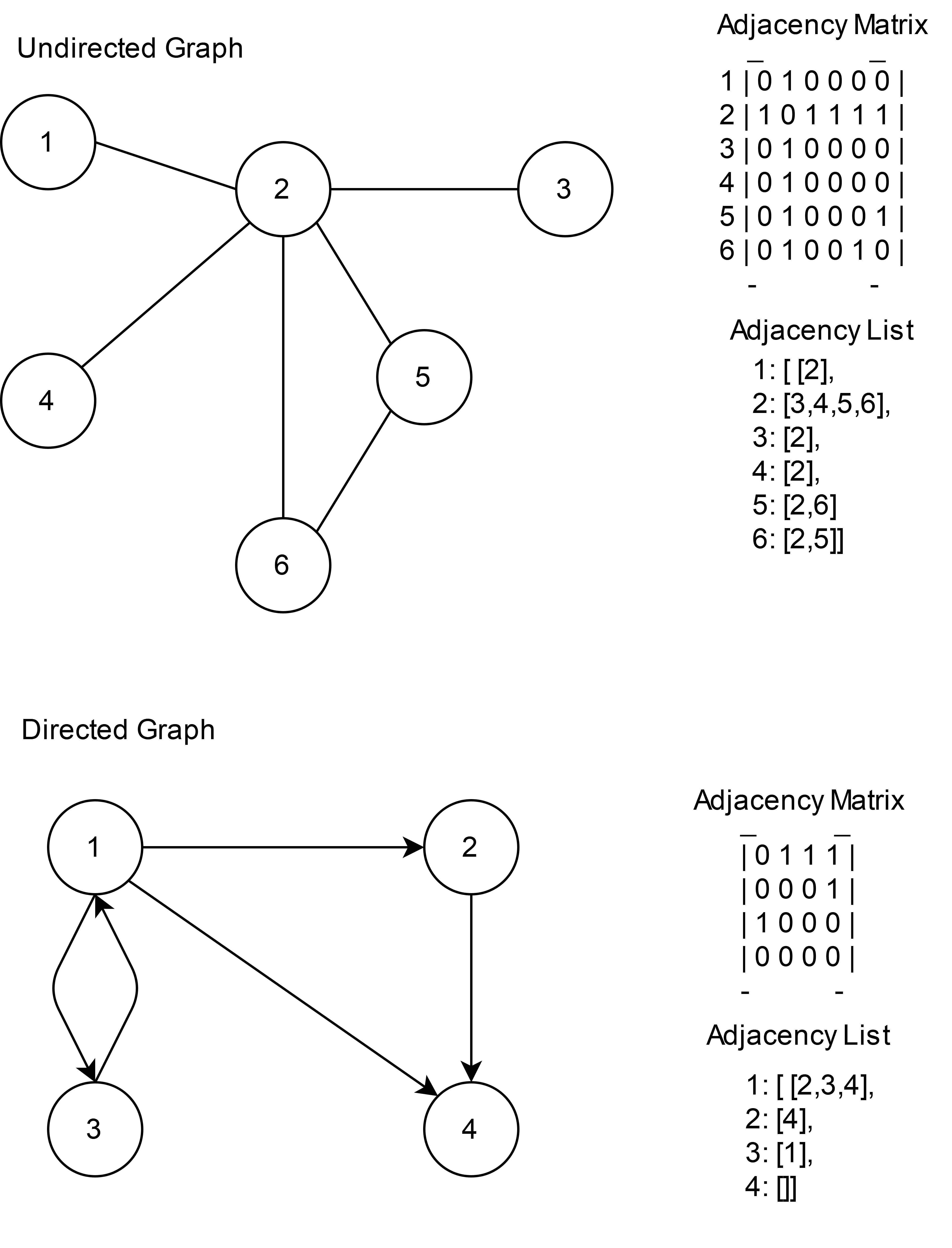
Depending on the algorithm we will use one of those representations.
Graph traversal#
Traversing a graph means visiting all if its nodes in some order. There are two basic algorithms to which achieve that goal.
Breadth-first search (BFS)#
The name of this graph traversal stems from the way it visits the nodes. It starts at some arbitrarily chosen node and then visits all the nodes that are distance 1 away from it, then distance 2 etc. BFS will not visit a node that is distance \(d+1\) until it visits all nodes at a distance \(d\). When two nodes are equal distance from the first node, the choice is also arbitrary (we will go for the numerical order).
Source: Wikimedia Commons
We will divide the nodes of the graph into three kinds: white, grey and black. White nodes are unvisited, grey are being considered and black are already visited. Grey nodes are a queue, first in last out. In words, the algorithm will work as follows:
Add all nodes to the white list.
Choose an arbitrary white node, put it in the grey queue.
Consider all nodes connected to the node, that are white, add them to the grey queue one by one.
Move the node considered to the black list.
If the grey queue is not empty, take another grey node and come back to the 3rd step.
If the white list is not empty, come back to the 2nd step, otherwise terminate.
The following implementations print the node id as they are added to the black list.
from queue import Queue
# adjacency matrix implementation
# indexing from 0, different from the diagram
def matrixBFS(graph):
    assert len(graph) and len(graph) == len(graph[0])
    white = list(range(len(graph)))
    grey = Queue()
    black = []

    # initalise the queue
    grey.put(0)
    white.remove(0)
    while True:
        # consider a node
        curr = grey.get()
        black.append(curr)
        # consider the nodes connected to the current node
        for i in range(len(graph[curr])):
            # add to grey if not previously seen
            if graph[curr][i] and i in white:
                grey.put(i)
                white.remove(i)
        print(curr)
        # check if all components if the graph is no connected
        # if all nodes checked terminate
        if grey.empty():
            for n in list(range(len(graph))):
                if n not in black:
                    grey.put(n)
                    white.remove(n)
                    continue
            if grey.empty():
                break

def listBFS(graph):
    assert len(graph)
    white = list(range(len(graph)))
    grey = Queue()
    black = []

    grey.put(0)
    white.remove(0)
    while True:
        curr = grey.get()
        black.append(curr)
        for i in graph[curr]:
            if i in white:
                grey.put(i)
                white.remove(i)
        print(curr)
        if grey.empty():
            for n in list(range(len(graph))):
                if n not in black:
                    grey.put(n)
                    white.remove(n)
                    continue
            if grey.empty():
                break
# Undirected
# 0   1
# | \
# 2 - 3
graph = [[0,0,1,1],[0,0,0,0],[1,0,0,1],[1,0,1,0]]
matrixBFS(graph)
print("")
graph = [[2,3],[0,3],[0,2],[]]
listBFS(graph)
print("")
# Directed
# 0    1
# /\ \  /\
# ||  \ |
# \/  \/|
# 2     3
graph = [[0,0,1,1],[0,0,0,0],[1,0,0,0],[0,1,0,0]]
matrixBFS(graph)
print("")
graph = [[2,3],[],[0],[1]]
listBFS(graph)
0
2
3
1

0
2
3
1

0
2
3
1

0
2
3
1
There are many uses of the BFS algorithm, some of which are:
Finding a MST (see below) in an unweighted graph.
Fining a minimum path in an unweighted graph (initial node has to be at the end of the searched path).
Detecting cycles in graphs (by encountering a visited node).
Finding all nodes within a connected component.
Depth-first search (DFS)#
In DFS we will always go deeper into the graph whenever possible. We start at an arbitrary node and then go to the first possible via an edge. This is repeated until we reach a node which has only edges to already visited nodes (or no edges). We then trace back to the previous node in this procedure. We continue until all nodes are visited.

Source: Wikimedia Commons
# DFS for matrix representation
def matrixDFS(graph):
    assert len(graph) and len(graph) == len(graph[0])
    # initalise
    white = list(range(len(graph)))
    black = []
    while white:
        root = white[0]
        white.remove(root)
        black.append(root)
        # recursive helper function
        DFShelper(graph,root,black,white)

def DFShelper(graph, root, black, white):
    for i in range(len(graph[root])):
        if graph[root][i] and i in white:
            white.remove(i)
            black.append(i)
            DFShelper(graph, i, black, white)
    print(root)

# Undirected
# 0   1
# | \
# 2 - 3
graph = [[0,0,1,1],[0,0,0,0],[1,0,0,1],[1,0,1,0]]
matrixDFS(graph)
print("")

# Directed
# 0    1
# /\ \  /\
# ||  \ |
# \/  \/|
# 2     3
graph = [[0,0,1,1],[0,0,0,0],[1,0,0,0],[0,1,0,0]]
matrixDFS(graph)
3
2
0
1

2
1
3
0
Time complexity of DFS is \(O(|V|+|E|)\). It can be used in the following problems:
Detecting cycles
Augmented DFS can find the MST of a graph
Minimum spanning tree (MST)#
A spanning tree of a graph \(G\) is a subgraph of \(G\) that includes all its nodes. The concept is meaningful for connected graphs only (if the graph is not connected we are considering its spanning forest). The problem of MST is considered for weighted graphs \((V,E\) with \(w\) - a function that returns the weight of an edge in \(E\). A minimum spanning tree is one in which the sum of weights of the edges is minimal. Surprisingly, the problem can be solved by using a greedy approach. Here are two possible approaches:
Kruskal’s algorithm#
Kruskal’s approach is based on the following procedure:
Create a single element set for every node.
Sort the edges in \(E\) by weight in non-decreasing order, put them in a priority queue.
Take the edge of least weight and if it connects elements from different sets, use it. Make the connected sets one (by setting the same group leader).
find(u) method will find the leader of a group. u,v are in the same group if find(u) == find(v).
union(u,v) will join two sets. The leader will be the leader of the set of more elements, otherwise arbitrary.
# we will use a matrix representation as a list of edges [source, dest, weight]
# we are also given the number of nodes
# assuming undirected graph
def mst_kruskal(edges,n):
    sets = {}
    mst =[]
    for i in range(n):
        # [leader, number of elems]
        sets[i] = [i,1]
    edges.sort(key = lambda x : x[2])

    for edge in edges:
        if find(edge[0],sets) != find(edge[1],sets):
            mst.append(edge)
            if union(edge[0],edge[1],sets) == n:
                return mst


def find(u,sets):
    # go up in parents
    while u != sets[u][0]:
        u = sets[u][0]
    return u

def union(u,v,sets):
    leader_u = sets[find(u,sets)]
    leader_v = sets[find(v,sets)]
    #compare which set is bigger
    if leader_u[1] >= leader_v[1]:
        leader_v[0] = leader_u[0]
        leader_u[1] += leader_v[1]
        return leader_u[1]
    else:
        leader_u[0] = leader_v[0]
        leader_v[1] += leader_u[1]
        return leader_v[1]

edges = [[0,1,6],[0,2,4],[1,5,3],[1,3,6],[0,4,7],[3,4,10],[0,3,1]]
print(mst_kruskal(edges,6))
[[0, 3, 1], [1, 5, 3], [0, 2, 4], [0, 1, 6], [0, 4, 7]]
Kruskal’s algorithm runs in \(O(|E|\log|E|)\) time, which is also \(O(|E|\log|V|)\) as \(|E| \leq |V|^2\).
Prim’s algorithm#
Prim’s algorithm is similar to Kruskal’s but at each step, there is only one tree that grows. The idea is as follows:
Start at an arbitrary node in \(G\)
Take the minimum edge incident on one of the already considered nodes (that connects it to the node not previously seen). This way the tree expands.
When all nodes are in the tree, terminate.
Of course, the 2nd step may be a bit tricky to implement efficiently. We will use a priority queue from the heapq interface to efficiently choose the next edge to add. We also need to upgrade our adjacency list representation of the graph. Now it is a dictionary which maps to a dictionary with incident nodes as keys and their corresponding edge weights as values. So graph[from][to] gives the desired edge if it exists. It assumes that there is at most one edge between any two nodes (undirected graph), if this is violated, we would always choose the edge of minimum weight.
from collections import defaultdict
import heapq

# we will work on an adjacency list representation
def mst_prim(graph, starting_vertex):
    # defaultdict returns set() in case the key is not in the dict
    # this is an adjacency list representation
    mst = defaultdict(set)
    # at the beginning only the starting_node is visited
    visited = set([starting_vertex])
    # get the edges incident on the starting_vertex
    edges = [
        (cost, starting_vertex, to)
        for to, cost in graph[starting_vertex].items()
    ]
    # create a min-heap based on the cost of the esge
    heapq.heapify(edges)

    while edges:
        # take the minimum cost edge
        cost, frm, to = heapq.heappop(edges)
        if to not in visited:
            # add the new node to the visited
            visited.add(to)
            # expand the tree
            mst[frm].add(to)
            # add the edges incident on the new node
            # which lead to the not visited nodes
            for to_next, cost in graph[to].items():
                # add to the heap
                if to_next not in visited:
                    heapq.heappush(edges, (cost, to, to_next))

    return mst

example_graph = {
    'A': {'B': 2, 'C': 3},
    'B': {'A': 2, 'C': 1, 'D': 1, 'E': 4},
    'C': {'A': 3, 'B': 1, 'F': 5},
    'D': {'B': 1, 'E': 1},
    'E': {'B': 4, 'D': 1, 'F': 1},
    'F': {'C': 5, 'E': 1, 'G': 1},
    'G': {'F': 1},
}

print(mst_prim(example_graph,'A'))
defaultdict(<class 'set'>, {'A': {'B'}, 'B': {'D', 'C'}, 'D': {'E'}, 'E': {'F'}, 'F': {'G'}})
The algorithm runs in \(O(|E|\log|V|)\) time. Why?
References#
Cormen, Leiserson, Rivest, Stein, “Introduction to Algorithms”, Third Edition, MIT Press, 2009
GeeksforGeeks, Applications of Breadth First Traversal
Vijini Mallawaarachchi, Medium, Towards Data Science, 10 Graph Algorithms Visually Explained, 2020
Brad Filed, Practical Algorithms and Data Structures, Prim’s Spanning Tree Algorithm, 2020